Airborne Lidar: A Tutorial for 2025

For a PDF which includes Tables click HERE

In recent years, both the miniaturization of sensors and advances in remote-controlled aerial platform technology have enabled the integration of scanning lidar (light detection and ranging) instruments into unmanned aerial vehicles (UAVs), also known as UAS (uncrewed aerial systems), RPAS (remotely piloted aerial systems), or colloquially referred to as drones. UAV laser scanning (ULS) delivers very dense 3D point clouds of the Earth’s surface and objects thereon like buildings, infrastructure, and vegetation. In contrast to conventional airborne laser scanning (ALS), where the sensor is typically mounted on a crewed aircraft, ULS utilizes UAVs as measurement platforms, which allow lower flying altitudes and velocities, resulting in higher point densities and, thus, a more detailed description of the captured surfaces and features.

Part I of this tutorial explained the fundamentals of laser ranging, scanning, signal detection, and the geometric and radiometric sensor models. While ALS and ULS are similar in the fundamental aspects of operation, the benefit of ALS is large-area acquisition of topographic data. In contrast, ULS can be thought of as close-range ALS. This facilitates applications which require high spatial resolution.

ULS is a dynamic, kinematic method of data acquisition. The laser beams are continuously sweeping in the lateral direction. Together with the forward motion of the platform, this causes a swath of the terrain and objects below the UAV to be captured. Distances between sensor and targets are determined by measuring the time difference between the outgoing laser pulse and the portion of the signal scattered back from the illuminated targets into the receiver’s field of view (FoV). Like laser scanning in general, ULS is therefore a sequentially measuring, active remote sensing technique.

In order to obtain 3D coordinates of an object in a georeferenced coordinate system (e.g., WGS84, ETRS89), the position and orientation of the platform as well as the scan angle must be continuously measured in addition to the distances. Thus, both ULS and ALS are kinematic, multi-sensor systems in which each laser beam has its own absolute orientation. The use of a navigation device consisting of a GNSS (Global Navigation Satellite System) receiver and an IMU (inertial measurement unit) is just as indispensable for ULS as it is for ALS.

ULS is a polar measurement system, i.e., a single measurement is sufficient to obtain the 3D coordinates of an object. This is particularly advantageous for dynamic objects such as treetops or high-voltage power lines, which are constantly moving owing to wind.

The ideal laser beam is infinitely small, but actual laser beams can be considered more like cones of light with a narrow opening angle (beam divergence). For ULS, typical diameters of the illuminated spot on the ground (footprint) range from cm to dm, depending on the flight altitude and beam divergence of the sensor. Due to the limited footprint, multiple objects along the laser line-of-sight can potentially be illuminated by a single pulse. In such a situation, sensors operating with the time-of-flight measurement principle can return multiple points for a single laser pulse. This so-called multi-target capability, combined with high measurement rates, results in unprecedented 3D point densities for the detection of semi-transparent objects such as forest vegetation (Figure 1) and power-line infrastructure.

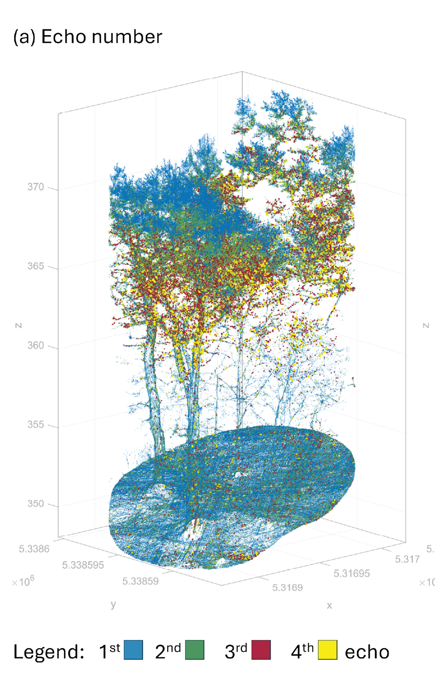
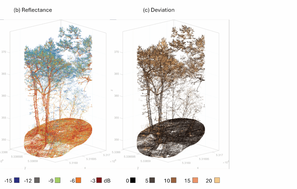
Figure 1: 3D UAV-lidar point cloud of a forest plot: (a) colored by echo number – 1st echoes (blue) accumulate in the canopy whereas 2nd, 3rd, and 4th echoes penetrate to the ground; (b) colored by reflectance – small twigs feature lower reflectance (blue) compared to laser returns from branches (green), and from stems and bare ground (orange, red); (c) colored by pulse shape deviation – dark/light color tones refer to high/low detection accuracy. Sensor: RIEGL VUX-10025.

In addition to signal runtime, ULS sensors typically provide additional attributes for each detected echo, with virtually all sensors returning at least the signal strength, also known as intensity. In particular, sensors which record the full echo waveform often also provide calibrated reflectance and detection quality indicators for each echo (Figures 1b and 1c). The strength of the backscattered signal depends on the laser wavelength used, which ranges from the visible green to the near-infrared part of the spectrum. Green laser radiation (λ=532 nm) can penetrate water and is therefore used in laser bathymetry to detect the bottom of clear and shallow waters, as discussed in Part III of this tutorial. Infrared wavelengths (λ=903/905/1064/1535/1550 nm), on the other hand, have better reflection properties for vegetation, soil, impervious surfaces, etc. Therefore, infrared lasers are the first choice for topographic mapping, forestry applications, infrastructure detection, etc.

Another similarity between ALS and ULS is data acquisition with partially overlapping flight strips. The overlap area forms the basis for (i) checking the strip matching accuracy and (ii) the geometric calibration of the sensor system through strip adjustment. ULS is particularly well suited for mapping corridors (river courses, narrow mountain valleys, forest transects, buildings in narrow street canyons, etc.). While manual control of the UAV is limited to visual line of sight (VLOS) operation, regular scan grid patterns are usually implemented via waypoints, which, with the appropriate authorization, also allow for beyond visual line of sight (BVLOS) flight.

The first commercially available UAV laser scanners appeared around 2015. At this time, ALS was already established as the prime method for capturing large-area terrain elevation data. While forestry and flood risk management were the driving forces for ALS around the turn of the century, it is nowadays predominantly the automotive industry which boosts sensor development. Indeed, since driver assistance systems make use of lidar sensors, this has promoted the development of low-cost sensors for the mass market. Many of these sensors are now integrated on to UAVs and used for 3D mapping. As a consequence, a broad range of UAV lidar sensors is available spanning from low-cost consumer-grade to high-end survey-grade instruments.

In the next sections, the different sensor concepts are introduced, followed by a discussion of the individual components, with respect to platform navigation as well as ranging and scanning. The tutorial concludes with a discussion of selected state-of-the-art sensors, examples of applications, and a list of related readings.

Sensor concepts

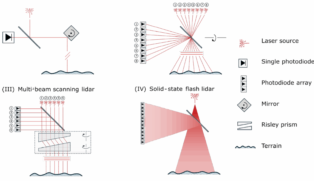
Figure 2: Schematic diagram of the various UAV lidar sensor concepts.

UAV lidar sensors can be divided into the following categories (Figure 2):

Single-beam scanning lidar
Rotating multi-beam profile array lidar
Multi-beam scanning lidar
Solid-state lidar

The basis of the first category is the conventional concept of linear-mode lidar systems, but with significantly reduced size and weight. With typical sizes of around 30×20 x20 cm and a weight of approximately 4 kg, these systems represent miniaturized versions of mature ALS sensors with a much smaller form factor and weight. Typically, a single high-class solid-state laser unit with a pulse repetition rate (PRR) in the MHz-domain is coupled with a rotating or oscillating beam deflection unit and a high-quality detector, typically consisting of an avalanche photon diode (APD) and a downstream AD converter, optionally with full-waveform digitization capabilities. These systems feature long measurement distances (~500 m) and provide high ranging precision (5-10 mm) as well as small and circular laser footprints with typical diameters of 5-8 cm when flown at 100 m above ground level (agl). To ensure eye safety, instruments in this class predominantly use near-infrared lasers with a wavelength of 1550 or 1064 nm.

Rotating multi-beam scanners do not have a beam deflection unit but use an array of diode lasers instead. All lasers fire at the same time with a single-beam PRR of 10-50 kHz. The laser beams form a fan with a typical FoV of 30°. The return signal of each laser is directed to an individual (silicon) APD receiver. The entire transceiver bundle rotates around a common axis, thus providing a 360° view. As multiple transceivers are employed, the quality of a single transceiver is lower compared to the transceiver unit of the conventional single-beam scanning lidar sensors. This applies to both the maximum measurement range and the laser beam divergence. Nevertheless, such sensor concepts are a core technology in the automotive industry for creating detailed 3D maps of a vehicle’s surroundings. This enables effective driver-assistance and even autonomous driving by precisely detecting and tracking objects. A major advantage compared to conventional survey-grade sensors is the much lower price. The alignment of multiple transceivers is a non-trivial task, however, especially for systems featuring more than 100 channels.

To mitigate the multi-channel alignment problem, a hybrid multi-beam scanning lidar concept was successfully established, which uses a few transceivers and a compact beam-steering device. Typically, six pulsed laser diodes and corresponding APD detectors are used as transceivers and beam deflection is implemented with a Risley prism, which consists of two (glass) wedge prisms that are arranged coaxially and rotate independently of each other around the optical axis. Depending on the current orientation of the wedge prisms, the laser beams are deflected differently due to refraction at the interfaces between glass and air. Depending on speed and direction of rotation, Risley prisms allow the creation of arbitrary scan patterns, ranging from straight lines via circles to spirals and floral patterns. The latter are used in the automotive industry to compile range images (3D scanning), again for driver assistance, collision avoidance, and fully autonomous driving. The former patterns (straight lines, shapes of a flat eight) are more suitable when such systems are mounted on UAV platforms, where 2D scanning is sufficient as the forward motion of the UAV provides the third dimension.

The last category is referred to as solid-state lidar, i.e. a concept without any rotating parts. The term “solid-state lidar” is used both for systems that use micro-electro-mechanical systems (MEMS) for beam deflection, and for so-called focal plane array systems, also referred to as flash lidar, which are comparable to digital cameras, where each pixel is a single APD and thus a single laser-ranging unit. APD arrays are common in Geiger-mode lidar, typically flown from very high altitude, but APD arrays can also be operated in linear mode and deployed on UAVs. Only focal plane array systems truly deserve the name solid-state, as there are indeed no moving parts. Regardless of brand of solid-state, however, the integration on UAVs is not widespread up to now.

From the above, it can be seen that there are significant differences between individual sensor components, ranging from low-cost consumer devices to high-quality surveying equipment. The following sections, therefore, discuss the core components of a UAV lidar sensor system, i.e., GNSS, IMU, laser range finder, and scanner, in more detail.

Platform positioning – GNSS

As discussed in Part I of the tutorial, 3D lidar points are obtained by direct georeferencing (cf. Part I, Equation 2), which combines platform position and attitude with laser scanner measurements. The positioning of the UAV is based mainly on global navigation satellite systems (GNSS), with data from various systems such as GPS, Galileo, GLONASS and Beido being used jointly today.

For UAV applications, GNSS is used twofold: (i) a base station with known coordinates in a well-defined reference system (e.g., WGS84 or ETRS89) serves as the basis for surveys with precisio in the cm range, and (ii) the UAV itself uses GNSS first to navigate to waypoints and fly predefined routes using real-time kinematic (RTK) corrections, either broadcast by the base station or by a GNSS network provider, and second to record the raw GNSS signals for calculating a single best estimate trajectory (SBET) in post-processing.

The GNSS device consists of an antenna and a receiver. For base stations, high-level choke-ring or radome antennae are used, which provide good multi-path suppression – this is important for ground-based installation. On the UAV, lighter and cheaper antenna types are used. Patch antennae are small and cheap and are therefore favored whenever accuracy demands are moderate. In most cases, helix antennae are used for UAVs. They have a typical cylindrical shape, and the actual antenna is a spirally wound wire. Helix antennae provide omnidirectional signal reception, which makes them susceptible to multi-path effects. This is not critical, however, as the platform is in the air. On the receiver side, either (i) single-, (ii) double-, or (iii) multi-frequency devices are available. This refers to the ability of the receiver to simultaneously receive the individual GNSS frequencies (L1, L2, L5). Obviously, multi-frequency receivers outperform single- and double-frequency devices, which in turn are cheaper. An important parameter is the measurement frequency. Today frequencies from 1 to 10 Hz are common. Manufacturers of GNSS devices for UAVs include uBlox and Septentrio (part of Hexagon), for example. Depending on the quality of the components, absolute coordinate uncertainties of the post-processed trajectory positions range from around 3 to 10 cm.

Platform orientation – IMU

Next to the position, the platform’s attitude must be precisely known at all times. IMUs continuously measure the platform’s motion using (i) gyroscopes, (ii) accelerometers, and (iii) optionally a magnetometer. Gyroscopes measure angular velocity (i.e. rotation rate) around three axes. Integration of angular velocity over time yields the actual orientation angles, e.g. roll, pitch and heading. Accelerometers, in turn, measure linear acceleration (i.e. velocity change), again along the three axes. Double integration of the accelerometer measurements yields positions with respect to the navigation frame (e.g., north/east/down): thus the IMU-accelerometer supports GNSS-based positioning. The optional magnetometer is used for correcting the heading angle with the Earth’s magnetic field. In general, IMUs feature a measurement frequency of 100-1000 Hz. The higher the IMU frequency, the better can high-frequency vibrations of the platform be captured.

In general, two different IMU concepts are in use: (i) fiber-optic systems and (ii) MEMS-based IMUs. Fiber-optic IMUs are more precise, but also more expensive and heavier. Therefore, MEMS-based IMUs are predominantly used for UAV-lidar, as they are compact, lightweight and cheap. Furthermore, the accuracy can be increased by rigorous calibration and by using multiple MEMS-IMUs in parallel. The accelerometers use tiny test masses suspended on springs, whose deflection is measured by capacitive sensors. The gyroscopes use vibrating structures (tuning forks) which experience a Coriolis force once the sensor/platform rotates. This results in a measurable displacement that is proportional to the angular velocity. Fiber-optic gyros, in turn, use light interference in the fiber bundle for measuring rotation rates.

No matter which technology is used, the final six degrees-of-freedom (6-DoF) trajectory consists of positions (x, y, z) and orientations (roll, pitch, heading) parametrized over time (t) and is achieved by fusing both GNSS- and IMU-measurements in post-processing, typically using Kalman filtering. The integration of GNSS observations is necessary, as IMUs provide only relative measurements, and the errors accumulate when integrating over time (drift). Achievable accuracies are in the range of 0.015° for the roll and pitch angles, 0.035° for the heading angle, and 2-5 cm for the position. In general, fiber-optic IMUs outperform MEMS-based IMUs with respect to accuracy. On the other hand, MEMS-based IMUs often provide higher measurement rates and are therefore better suited to capture high-frequency platform movements.

Ranging

In Part I of this tutorial, we discussed the general principle of laser ranging in detail and concluded that distinct laser echoes are either detected directly within the receiver electronics based on trigger thresholds (discrete echo systems) or by digitizing the entire backscattered echo pulse and detecting individual echoes within the sampled full echo waveform. The latter can be done either online in the instrument or in post-processing, if the waveform is additionally stored on disk. Both technologies are also available for UAV-lidar. Survey-grade single-transceiver instruments often operate based on full-waveform digitization, while multi-beam sensors tend to use discrete echo detection.

A major difference between survey- and consumer-grade sensors is the laser technology used. Typically, ranging can be conducted using relatively cheap diode lasers and more expensive solid-state lasers or fiber lasers. Diode lasers, frequently used in the automotive industry, emit laser radiation at a wavelength of 905 nm (near-infrared). The advantage of using this wavelength is that standard silicon detectors can be used, which makes the lidar sensors cost-effective. With respect to eye-safety, the use of a longer wavelength, e.g. the 1550 nm produced by the erbium-doped fiber laser, is beneficial as more laser power can be used without compromising eye safety. This is especially relevant for UAV-lidar as the sensors are operated close to the ground with typical flying altitudes of around 100 m agl. Nevertheless, the use of a 1550-nm laser implies the use of expensive InGaAs photodiodes. For this reason, fiber lasers are used only in survey-grade UAV-lidar sensors, which offer higher peak power, better beam quality, smaller beam divergence, higher PRR, and potentially lower pulse duration, in exchange for the higher cost. Diode lasers, in turn, are not only cheaper but also more compact, which is relevant as payload is of great concern for UAV-lidar.

Scanning

As with conventional ALS, UAV-lidar also captures the Earth’s surface based on flight strips. For single- or multi-beam scanning lidar systems, areal coverage with 3D points requires (i) the forward motion of the UAV platform and (ii) a beam deflection unit systematically steering the laser rays below or around the sensor. Figure 3 shows some of the typical beam deflection mechanisms used in ULS.

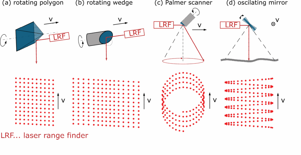
Figure 3: Strategies for laser beam deflection used in single-beam scanning UAV-lidar.

If scanning is performed in a vertical plane, rotating polygonal mirrors operated with a constant speed produce a linear point pattern on the ground with equal point spacing in the nadir direction and slightly increased spacing at the strip boundary. Depending on the number of mirror facets (2-4), a FoV of 60-160° is achievable. Interesting variants are available on the market, where the individual mirror facets are slightly tilted, enabling forward, nadir and backward looks in a single revolution of the mirror wheel, which is especially beneficial for scanning vertical structures and (semi-transparent) vegetation. Rotating mirrors also allow panoramic scanning (FoV=360°) using a single mirror facet tilted by 45°. Oscillating mirrors constantly swing between two positions and produce a zigzag pattern on the ground, with the slight disadvantage of a less homogenous point distribution, especially at the strip border, due to the deceleration and re-acceleration of the mirror. Conical (Palmer) scanning is also used in UAV-lidar, notably for UAV-based laser bathymetry (cf. Part III of this tutorial).

Risley prisms use ray refraction at the air-glass-air interfaces for beam steering, as opposed to reflection at a mirror surface. Risley prisms are used in the family of hybrid multi-beam scanning lidar sensors. As stated before, the two beveled glass wedges of the Risley prism can be operated independently and produce arbitrary scan patterns. In the UAV context, however, the predominant scan pattern resembles a flat figure-of-eight loop. This causes the laser beam’s line of sight to be directed slightly forward and backward at the edge of the strip and almost towards the nadir in the center of the strip. The disadvantage of refraction-based beam steering is that scattering in the glass slightly deteriorates the beam quality. Figure 4 shows the sensor and scanning concept of the Livox Avia instrument, a representative multi-beam scanning lidar instrument.

Figure 4: (a) lidar and scanning unit of the Livox Avia multi-beam scanning lidar; (b) and (c) ground plan and perspective view of the object points during a full rotation of the scanning unit (six parallel figure-of-eight loops).

Finally, no distinct beam deflection unit is necessary for multi-beam profile-array scanners and solid-state flash lidar systems. For the former, the entire transceiver bundle rotates 360° around a common axis, which for UAV-integrations is either horizontal or slightly tilted. This kind of panoramic scanning is beneficial for scanning narrow street canyons or narrow valleys as it allows capturing 3D points both below and above the platform.

Examples of sensors and integration

Table 1 (see PDF) lists the specifications of selected commercially available UAV lidar sensors, extracted from the data sheets published by the individual manufacturers.

The table lists a series of survey-grade single-beam scanning lidar sensors (category I) from various manufacturers with a measurement precision below 1 cm (VUX1-UAV, VUX-120, CL-360HD2, CL-90, Zenmuse L3, H600, TrueView540). All these sensors use a high-class 1535- or 1550-nm laser and a corresponding high-quality receiver. from 160 to 2000 m, depending on instrument and pulse repetition rate. For these instruments, the latter is in the range of 100 kHz to 2.4 MHz. Devices with high PRR, in excess of 2 MHz, also offer measurement modes with reduced pulse frequency, whereby the maximum measurement distance is extended due to the higher laser power available for a single laser pulse. The survey-grade instruments also provide the smallest beam divergences (0.3-0.5 mrad), yielding a small laser footprint on the ground of 15-25 mm.

The rotating multi-beam profile array sensors (PuckLITE, Alpha Prime; category II) and the multibeam scanning lidar sensors (Avia, Zenmuse L2; category III), in turn, are typically lighter than their category I counterparts. The Zenmuse L2, for example, weighs less than 1 kg, including IMU and a 20 MP RGB camera. These systems all use 905-nm diode lasers. They typically exhibit low beam divergence in one direction and higher divergence in the orthogonal direction, which leads to elliptical footprint areas on the ground. The achievable spatial resolution is limited by the larger of the two diameters as well as by the point-to-point distances. The latter depends on the PRR, the rotation speed of the scanning unit or the laser bundle, and the flying altitude. A typical feature of multi-beam sensors is that the pulse rate of a single laser source is moderate (2-40 kHz), but the resulting net pulse rate can be high due to coupling multiple channels. The AlphaPrime, for example, has a pulse frequency of 2.4 MHz, which results from 128 channels, each with a PRR of approximately 20 kHz.

Table 1 also lists three topobathymetric UAV laser scanners (Navigator, VQ-840-GL, VUX-820-G), which use a green laser at 532 nm. All three are category I instruments (single-beam scanning lidar) and feature full-waveform digitization, which is obligatory for bathymetric scanners. For eye-safety reasons, these systems have a relatively large beam divergence of 4 mrad (Navigator) or 1–6 mrad (VQ-840-GL). In all cases, the devices must be operated in such a way that the nominal ocular hazard distance (NOHD) is maintained. This means, for example, that operating the VQ-840-GL with a beam divergence of 1 mrad requires a certain minimum flight altitude (>120 m agl).

All the listed sensors are typically mounted on multicopter UAV platforms and operated in VLOS mode, i.e. with permanent sight contact between pilot and UAV. Depending on the total payload, today’s multicopters allow flight times of around 20-45 minutes with one battery set. When the integration is on fueled aircraft and operated in BVLOS mode, much longer flight endurance is possible, opening the way for large-area 3D mapping in high resolution. This applies to all possible aerial systems including multicopters, helicopters, fixed-wing UAV, and systems supporting vertical takeoff and landing (VTOL). Figure 5 shows an example of integrations of two different UAV-lidar sensors on the same multicopter platform.

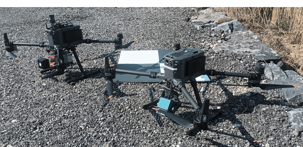
Figure 5: Integration example: RIEGL miniVUX-3UAV (left) and DJI Zenmuse L2 (right), each mounted on a DJI Matrice 350 RTK multicopter UAV.

Application examples

The main advantages of UAV-lidar over conventional ALS from crewed aircraft are (i) the higher spatial resolution and (ii) the lower mobilization costs. These come at the expense of limited area coverage due to limited endurance, lower flight altitude entailing smaller swath widths, and lower flight speed. Thus the use of UAV-lidar is always economical when the size of the area of interest is moderate and when repeat data acquisitions are required to capture processes.

The fields of application include:

3D mapping of topography and shallow-water bathymetry
3D mapping of urban scenes including as-built 3D documentation of construction sites (houses, bridges, dams, etc.)
3D vegetation mapping (forest extent, forest structure, biomass estimation, tree species classification, diameter at breast height derivation, urban vegetation, etc.)
3D mapping for monitoring of natural or artificial processes including landslides, rockfalls, avalanches, glacier retreat, hydro-morphological changes, open pit mining, etc.
3D corridor mapping including powerlines, railways, motorways, creeks in steep alpine terrain, etc.
Archaeology, especially detection and documentation of remains hidden under vegetation canopy or submerged in lakes or the sea
Ecology, especially detection of standing and lying dead wood, high-resolution wetland mapping, identification of ecological niches, etc.
Agriculture, especially in the context of precision farming, to monitor plant growth and phenology

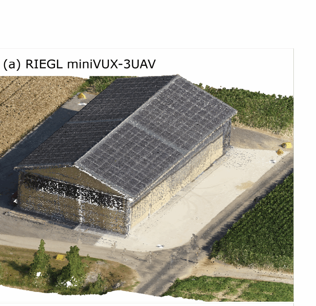
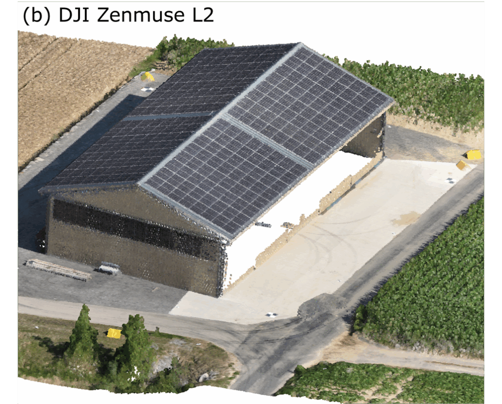
Figure 6: 3D RGB-colored UAV-lidar point cloud of an agricultural warehouse captured with (a) RIEGL miniVUX-3UAV and (b) DJI Zenmuse L2.

Figures 6-9 are results of UAV-lidar applications. Figure 6 shows an agricultural warehouse captured with two different sensors, a single-beam 360°-scanning lidar and a multi-beam scanning lidar with 75° FoV. Both sensors capture the warehouse and its surroundings and also provide RGB-colored point clouds based on the integrated cameras. The 360° scanner provides better coverage of the vertical walls. This could be compensated, however, by tilting the multi-beam scanner sideways, which is supported by the instrument.

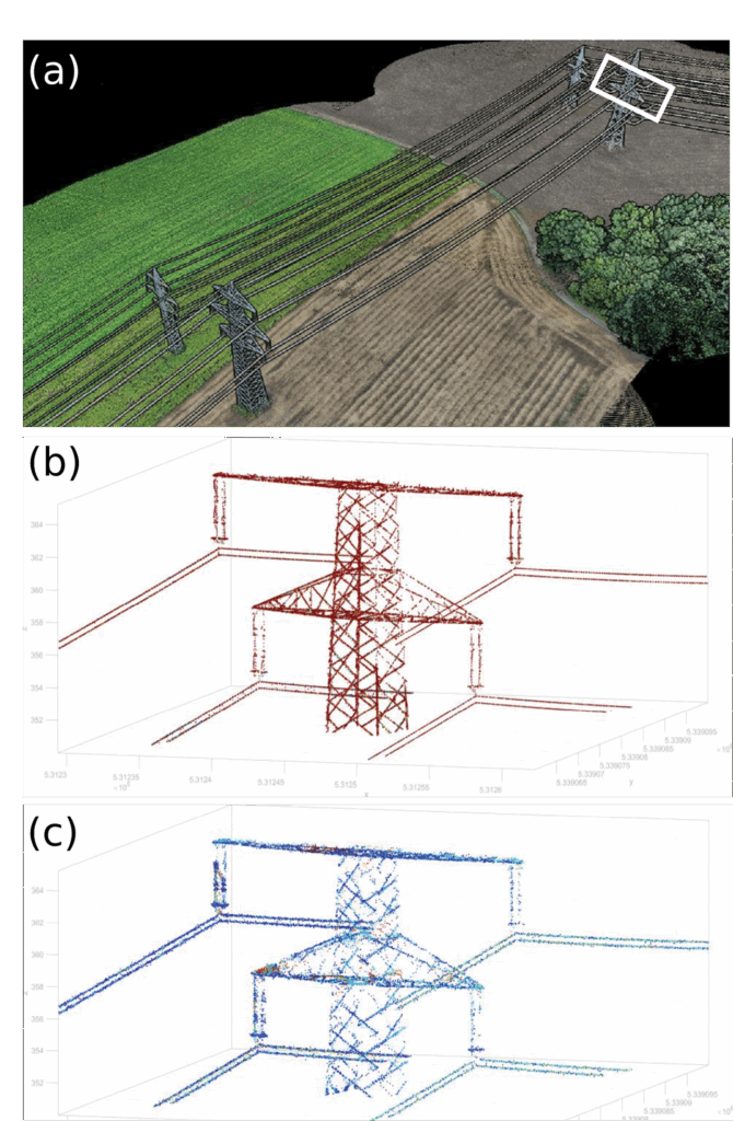
Figure 7: (a) True-color 3D point cloud of a double-track high-voltage power line captured with the DJI Zenmuse L3 laser scanner. The white rectangle marks the detail shown in: (b) Zenmuse L3 (September 2025) and (c) Zenmuse L2 (August 2024).

Figure 7 shows the 3D point cloud of a double-track high-voltage power line and provides an example of corridor mapping. The scene shows points on the individual cables and power poles, but also details such as insulators, which can normally only be captured with terrestrial laser scanning, but are well resolved with a compact short-range UAV-lidar.

Figure 8: (a) True-color 3D point cloud of the Pielach River captured in July 2025 with the YellowScan Navigator topobathymetric laser scanner; (b) cross-section with points colored according to classification.

Figure 8 showcases topobathymetric UAV-lidar. The scene, from the pre-Alpine Pielach River in Lower Austria and the surrounding alluvial forest (nature conservation area Neubacher Au), was captured with an integrated sensor consisting of a topobathymetric lidar unit and an RGB camera. The detail in Figure 8 shows a representative section of the point cloud classified into dry and submerged ground, water surface, water column, and vegetation resulting from data post-processing in the manufacturer’s software.

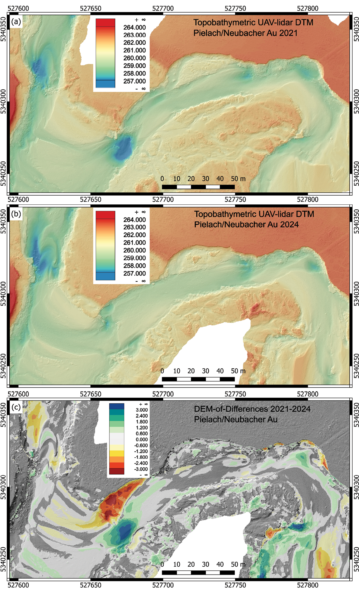
Figure 9: Color-coded and shaded DTMs of a section of the Pielach River captured twice, (a) in 2021 and (b) after a major flood in 2024, with the RIEGL VQ-840-G topobathymetric laser scanner; (c) color-coded DEM-of-differences map showing clear erosion and deposition patterns.

Finally, Figure 9 shows DTMs of same area captured twice in 2021 and after a major flood in 2024 with a different topobathymetric UAV-lidar system. Both datasets were rigorously georeferenced using a permanent local GNSS base station so that the DEM-of-differences shows the enormous impact of the September 2024 flood event, with total erosion (yellow to red) and deposition (green to blue) of 3600 m3 and 5100 m3, respectively. Data post-processing was carried out with the manufacturer’s software and with the scientific laser-scanning software OPALS developed at TU Wien.

Concluding remarks

This concludes the four-part tutorial on airborne lidar for 2025. Part I discussed the basics of airborne lidar and introduced the fundamental formulae (ranging, laser-radar equation, direct georeferencing). Part II focused on integrated systems consisting of active lidar and passive camera sensors as well as on multispectral lidar. The general topic of Part III was laser bathymetry using water-penetrating green lasers. And, finally, Part IV provided details on UAV-lidar, which is a rapidly growing field.

I would like to thank all readers for their attention, comments, and feedback. I hope that some readers of LIDAR Magazine will find this compact tutorial useful. Please don’t hesitate to contact me if you have any questions. I will be happy to discuss them with you. Finally, I would like to express my gratitude to the magazine team—especially Stewart Walker—for giving me the opportunity to write this tutorial. Thank you for your trust.

Dr. Gottfried Mandlburger studied geodesy at TU Wien, where he also received his PhD in 2006 and habilitated in photogrammetry with a thesis on “Bathymetry from active and passive photogrammetry” in 2021. In April 2024 he was appointed University Professor for Optical Bathymetry at TU Wien.

His main research areas are airborne topographic and bathymetric lidar from crewed and uncrewed platforms, multimedia photogrammetry, bathymetry from multispectral images, and scientific software development. Gottfried Mandlburger is chair of the lidar working group of Deutsche Gesellschaft für Photogrammetrie und Fernerkundung, Geoinformation e.V. (DGPF) and Austria’s scientific delegate in EuroSDR. He received best paper awards from ISPRS and ASPRS for publications on bathymetry from active and passive photogrammetry.