Figure 1: SATW fact-sheet. Image courtesy of SATW.
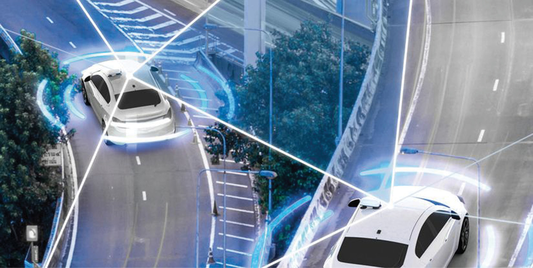
The Swiss Physical Society (SPS) intermittently publishes short reports on events or publications of the Swiss Academy of Engineering Sciences (SATW). Recently SATW produced a fact-sheet on autonomous mobility (Figure 1)2. It describes the future of driving fully autonomous cars. Already enthusiastically hailed by many as an important historical milestone, autonomous driving is also perceived by some as an unnecessarily wasteful and overly expensive endeavor by major industries, ignoring the more urgent problems of our time. But there are many positive arguments, such as a reduction in the number of accidents and an increased mobility for the disabled, elderly persons and children.
Editor’s note: A PDF of this article as it appeared in the magazine is available HERE.
Where do we stand today? And where is development heading? The fact-sheet comments in tabular form on the developmental stages of autonomous driving (3 = conditional automation, 4 = high automation and 5 = full automation) on the basis of criteria such as technical challenges, individual and social benefits, risks, social acceptance, legal aspects and estimated time horizons.
Key messages
The study assumes that, despite all concerns, the development of autonomous driving will continue worldwide and at great expense, simply because a phalanx of major technology and service companies see this as the key market of the mobility business. The rapidly growing technological possibilities in digitization, algorithms, networking and communication can be bundled and developed into sophisticated industrial activities—it is an opportunity that no modern nation can pass up.
On the other hand, the SATW study does not ignore the fact that the challenges facing the implementation of autonomous driving are so great that market penetration with partially or highly automated vehicles is not expected for at least twenty years, and fully autonomous vehicles will be on the market in about forty years. The difficulties are significant because, among other things, safety issues are paramount and collisions between passers-by and vehicles depend on so many factors—technical, environmental or psychological—that they cannot yet be sufficiently identified and evaluated.
High complexity
In order to get a feeling for the enormous complexity of this automated vehicular undertaking, we cite a lecture on 12 June 2018, at the Technology Day of the University of Applied Science NTB in Buchs, Switzerland. A representative of a large automobile engineering company spoke about “new and integrated active chassis systems for future vehicle concepts”. He mentioned that the software currently installed in a car will increase from 100 million lines of code to 200 billion in 2030. That would still be at level 4! Since the software will consist of many submodules, the consistency of all interfaces must be guaranteed—this
is a very demanding task.
Equally thought provoking is the testing effort: “to prove safety with 95% confidence [needs] eight billion km of road testing [with] 100 vehicles 24/7 for 225 years”. This is a troubling statement at a time when safety margins in many areas such as the space industry require at least eight sigma. Can (cyber-)physics help here?
Mini-Trams
The main problem is the unmanageable variety of possible interactions between vehicles but also between vehicles and pedestrians. How would a physicist proceed? One would first set meaningful boundary conditions, then carefully measure and finally compare experimental results with physical models, thus minimizing deterministic and stochastic errors.
Meaningful boundary conditions are those that acceptably limit the performance requirements. When driving autonomously, what counts primarily is the permanent availability of vehicles that drive individually, safely and comfortably to a home address, but not, for example, the maximum speed or a minimum distance between vehicles.
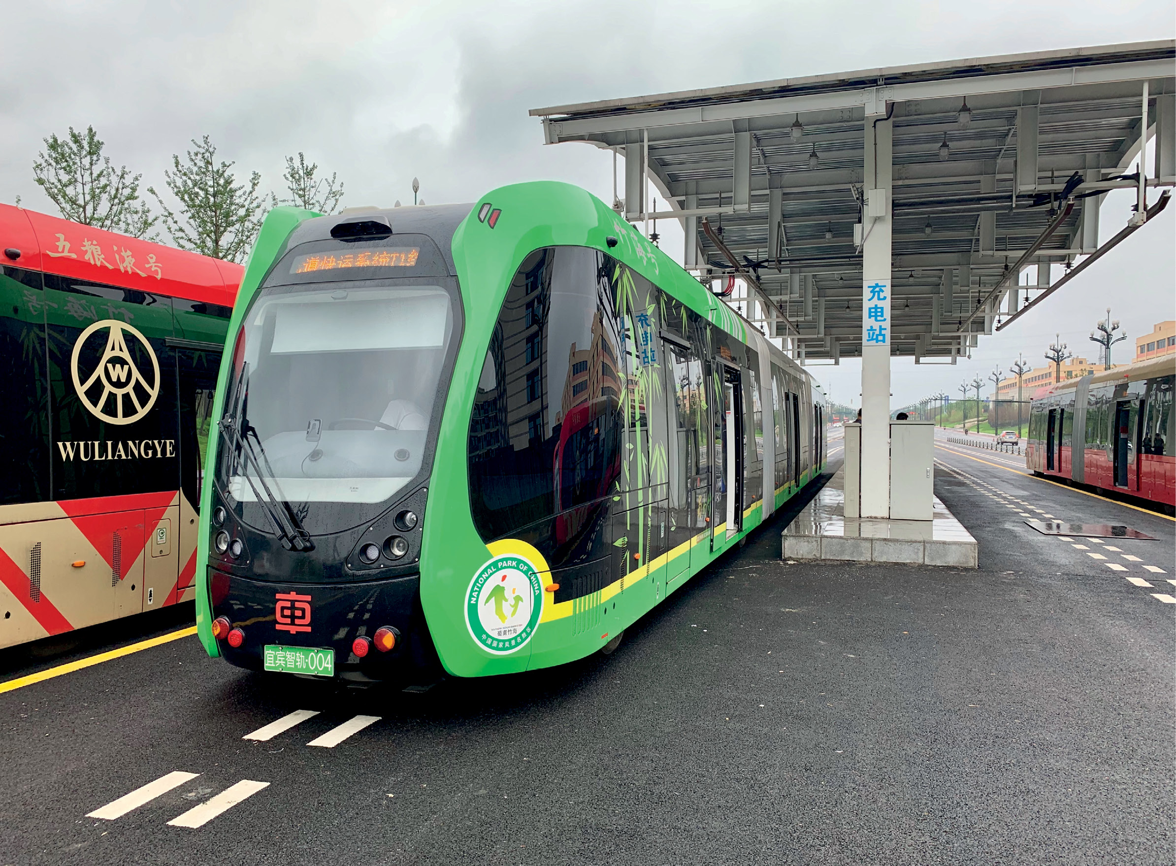
Figure 2: Trackless tram in Zhuzhou, China. Source: https://commons.wikimedia.org/w/index.php?curid=79705921.
Thus, one could consider autonomous mini-trams in regular traffic, running on tracks at a constant speed. This sounds rather unrealistic, but in the city of Zhuzhou in China whole tram trains are already running on normal main roads without rails, guided only by marked lines and stationary sensors at the roadside (Figure 2).
Stationary sensors are not a viable solution for regular road traffic, however, where driving on dense networks of secondary roads and side streets has top priority. For cost reasons alone, only vehicle-mounted sensors should be used—in combination with stationary global systems such as satellite navigation. But even sensors should only play a supplementary role, because the most obvious and safest solution would be to replace the usual road markings with weatherproof and physically optimized special paints that serve to guide the vehicle by means of suitable optical and magnetic sensors. Magnetic guidelines are already known from their use in factories, but using them in road traffic is probably somewhat novel. Road marking is simple, inexpensive, proven and tested, and it would cover all the streets of a particular city, including the suburbs, without restricting traditional, non-autonomous traffic.
This guidance would still need support by onboard GNSS, INS, LOPS, lidar and image processing sensors, which we describe briefly. A good summary is available online3.
GNSS (Global Navigation Satellite Systems)
Various satellite systems can be used for navigation: GPS (USA), Glonass (Russia), Galileo (EU), Beidou (China), IRNSS (India) and QZSS (Japan). Direct positioning is accurate only to about ±10 m due to satellite errors (residual clock errors, orbit variations), dispersion effects in the ionosphere and troposphere, as well as multiple reflections off buildings and trees. In addition to technical measures such as the transmission of satellite signals in various frequency bands to eliminate frequency-dependent dispersion errors, complex configuration concepts such as DGNSS, SBAS and RTK reduce the error rates so that accuracies of only a few cm can be achieved. At the same time, the stability and robustness of position measurement has been much improved in recent years, together with a shorter acquisition time before measurements with cm accuracy are available. While a few years ago one had to wait up to one hour for the highest accuracy level, today it takes only a few seconds. To achieve these cm accuracies for a moving vehicle (called a ‘rover’), the following approaches are used:
Differential GNSS (DGNSS)
A stationary GNSS station (base) calculates its actual position from the satellite data and compares it with its true position, which has been accurately measured previously using land surveying techniques. The deviations, caused by the aforementioned errors, are sent via radio link to the mobile rovers, which correct their position calculations. The position determination is based on the correlation of the transmitted code sequences of the satellites that are used.
Satellite based augmentation systems (SBAS)
Within a larger region, it is more cost-effective to replace the individual base stations with a network of stationary and accurately known GNSS receivers. These continuously send their calculated position data to a central station. There the current correction data for each point in the region is calculated and sent to special geostationary SBAS satellites that retransmit it over the region. Every rover in the region can thus obtain the correction data valid for its location online.
Real-time kinematic (RTK)
Similar to DGNSS, a stationary base station is used as reference, which sends the correction data it calculates to each rover via radio link. The difference from DGNSS is that instead of code correlations, more computationally complex analyses of the code phases are carried out when determining the position. This leads to position accuracies of ±1-2 cm.
INS (Inertial Navigation Systems)
While the velocity and acceleration vectors can be derived with high accuracy from the position measurements of a GNSS sensor by differentiation, the determination of tilt angles is poorly conditioned. It is therefore better to measure them directly, especially if one wants to set certain tilt angles (tilting trains) or to compensate or damp stochastic tilt errors as in ships or aircraft.
INS sensors measure the linear accelerations and, by means of gyros, also measure the angular accelerations in the three main axes. Since the position and angles (roll, pitch and yaw) are obtained from the measured accelerations by double integration, the INS system can take over the function of the GNSS sensors in case of a temporary failure. On the other hand, the GNSS sensors, which measure absolute positions, can monitor the behavior of the two integration constants of the INS system. For mapping applications that use airborne photogrammetry and lidar, the sensitive position of the aircraft is monitored by INS sensors with a high clock rate of 200 Hz, whereby their zero drift is corrected by GNSS systems with a lower clock rate.
LOPS (local optical positioning system)
This optical method is similar to GNSS, except that the rover is both code emitter and code receiver. The rover sends code-modulated signals to its chosen ‘satellites’ and measures the distances together with the two polar emission angles in its own coordinate system. Since LOPS uses laser light as code carrier, the optical ‘satellites’ are prisms or foils, but also highly reflective spots on objects like buildings. If one knows the exact positions of the reflectors in a local urban coordinate system, then the 3D current position and angular orientation of the rover can be determined by triangulation and compared with the GNSS measurements. Since the reflectors are passive and that the only time base is at the rover, one needs only three, not four reflectors. Combining GNSS as a passive global sensing method with LOPS as an active one can ameliorate problematic situations, such as the corruption of the GNSS data by fake signals produced by simple electronic devices, which must be immediately identified and eliminated to avoid serious disasters by misguiding. LOPS systems on vehicles can permanently change the code modulation of their lidar beams, so that their 3D-scan information of the environment (buildings, cars, etc.) is robust against attacks. Furthermore, LOPS can identify stationary or mobile objects which can scatter the GNSS signals: this again helps to improve and accelerate the GNSS algorithms4.
Lidar
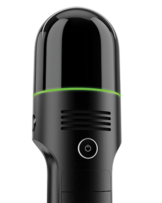
Figure 3: Leica BLK2GO handheld imaging laser scanner. Image courtesy of Leica Geosystems.
In lidar systems, laser beams are modulated in amplitude and phase (similar to GNSS signals) in such a way that distances can be measured. The 3D acquisition of a scene can be done by laser scanning or by sending out a fixed bundle of laser beams, called an “image ranger”. Lidar systems built into vehicle headlamps can detect objects in the driver’s field of view as well as determine their own position and orientation by scanning the environment. Figure 3 shows a modern lidar system from Leica Geosystems, in which an eye-safe laser scanner captures objects from 0.5 m to 25 m or even up to 60 m away with a resolution of about 8 mm at clock rates of about 400 kHz. Integrated wide-angle and IR cameras as well as INS modules support the lidar system.
Line-Marking
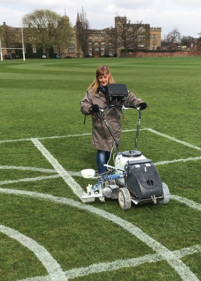
Figure 4: Views of GNSS-guided line-marker. Images courtesy of Fleet Line Markers Ltd.
How well a vehicle can be guided by means of marked lanes and GNSS sensors is demonstrated by a reverse variant, namely the line-marking of roads and (sports) arenas by means of GNSS and INS sensors and the use of stochastic estimation algorithms. In the line-marker shown in Figure 4, the spray nozzle is mounted on a motor-driven spindle, the position of which is guided transversely to the direction of travel, so that the line is marked without jittering in spite of driving errors and terrain irregularities5. Given a stationary RTK base station, line curves of any kind can be marked over areas with side lengths of several hundred meters, whereby several semi- or fully automated rovers can be in operation at the same time. Figures 5 and 6 provide more detail. The RTK GNSS signals, together with the data from an INS sensor, are fed into a Kalman-filter algorithm, the predicted values from which are used to control the nozzle position.
Algorithms
The high performance of algorithmic estimation methods shown in the line-marking example could also help to ease the problem of erratic pedestrian behaviour. It is certainly not enough to be able to recognise from a vehicle that a person might cross the road, but how would she or he behave afterwards? A child is more likely to jump spontaneously into the street, but would just as quickly come back again, while an elderly person would only hesitantly step into the road, but would then react slowly in the event of a dangerous situation. It can be assumed that in the coming years it will be possible to anonymously query the movement profiles of a person at the side of the road, via mobile phone, smartwatch or health wristband, from the vehicle for a few seconds in order to predict the next step and vice versa. It is imperative, however, that the data be immediately deleted after the prediction.
Cyberphysical systems: digitization, artificial intelligence, new networking technologies and their physical modeling
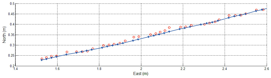
Figure 6: Extract from a measurement series for a straight line. The measured values, plotted in the east and north directions, show the movement of the line-marker at a deliberately slow driving speed of about 1 m/s. The red points are the GNSS positions (clock rate 20 Hz) with a variation of about ±1-2 cm, with which the line can be marked with acceptable quality. If the data is combined with the INS measurement values and fed into a Kalman-filter algorithm, however, the position of the spray nozzle is controlled according to the blue curve with deviations of only few mm from the ideal line. Image and measurement data courtesy of Braunecker Engineering GmbH.
As mentioned in the SATW fact-sheet, the above modern technological approaches are becoming increasingly powerful. A skillful combination of these will help reduce possible conflict situations for autonomous vehicles and characterize them by means of a kind of cataloging. Meaningful boundary conditions such as the use of guidelines with physically optimised paint properties, as well as sensor fusion combined with powerful adaptive algorithms, will significantly reduce the degree of complexity. Instead of extensive and ultimately irrelevant test drives over many villages, potential conflict situations could then be reliably modelled, simulated and verified in local test facilities, so that the results are applicable anywhere and at any time. The reliability of the measurements and their allocation then allows suitable countermeasures such as warning, braking, evasion, etc. to be taken in real situations.
1 Dr. Braunecker provided some input to our recent piece by Allen Cheves and Stewart Walker, “Schott at the sharp edge”, LIDAR Magazine, 10(4): 6-12, Fall 2020. During the correspondence he suggested that we could publish the present article, which has already appeared in German: Braunecker, B., 2020. Cyberphysische Systeme und Autonome Mobilität, SPG Mitteilungen, 61, 44-46, June. As editor of SPG Mitteilungen, Dr. Braunecker gave us permission to publish it. Our version is based on an English translation available on the SPS website. We have made minor modifications to suit the style of LIDAR Magazine.
4 United States Patent US 7,742,176 B2 (22 June 2010), Braunecker et al.