For a PDF which shows the table and the formulas click HERE
With the geospatial industry increasingly moving towards three-dimensional GIS and true three-dimensional representation of terrain and infrastructure, it becomes prudent for mapping standards to provide a measure to assess the accuracy of such representations. This measure was defined in the latest American Society for Photogrammetry and Remote Sensing (ASPRS) Positional Accuracy Standards for Digital Geospatial Data, published in 2024, in which the term “three-dimensional accuracy” was introduced to complement horizontal and vertical accuracy terms. This article provides users of the standards with practical methods for assessing the three-dimensional accuracy of geospatial data and helps them understand this new term of accuracy.
Our world in 3D and the challenges in representing it
Whether from space or aerial platforms, advances in lidar, radar, and other mapping and surveying sensors and instruments enable us to view the world in true 3D—revealing what we have never seen before. GIS, environmental, and engineering applications are becoming heavily dependent on 3D point clouds and 3D modeling (see Figures 1 through 3). Similarly, new applications like digital twins, BIM, and smart cities push the demands for 3D data to a new level.
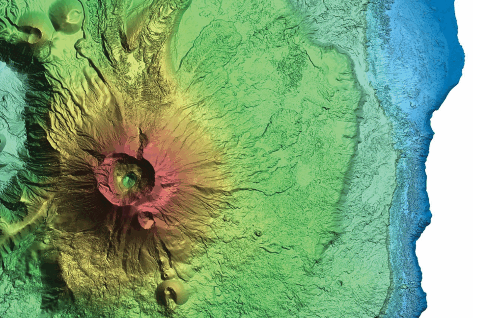
Figure 1: Lidar model of a volcano site in Hawaii. Courtesy of Woolpert and USGS
Despite the high demand for 3D data, the industry is still behind in dealing with such data in a true 3D environment. We are still evaluating horizontal and vertical accuracy separately owing to the lack of effective tools for visualizing and performing measurements in 3D. Even the most widely used GIS and CAD tools in the industry do not provide such capabilities. What badly need software manufacturers to create a tool that presents 3D models or point clouds in true 3D and provides a terrain-following cursor for 3D measurement capabilities.
The new 3D positional accuracy
The ASPRS Positional Accuracy Standards for Digital Geospatial Data, Edition 2, Version 2 (2024) provides the following justification for introducing the new third term of positional accuracy: “Three-dimensional models and digital twins are gaining acceptance in many engineering and planning applications. Many future geospatial datasets will be in true three-dimensional form; therefore, a method for assessing positional accuracy of a point or feature within the 3D model is needed to support future innovation and product specifications.1”

Figure 2: 3D model of an industrial complex. Courtesy of Woolpert
According to the standards, the accuracy of the 3D position (X, Y, and Z) of features, with respect to horizontal and vertical datums, is computed using the following formula:
The RMSEX, RMSEY, and RMSEZ of the checkpoints are computed by comparing the coordinates obtained from the map or 3D model to the surveyed coordinates of the checkpoints.
Suggested strategy to quantify the 3D accuracy
The following are scenarios that users may encounter when assessing 3D positional accuracy:
1. Using checkpoints that are suitable for vertical and horizontal accuracy assessment
These checkpoints are usually referred to as photo-identifiable checkpoints. Users can easily identify and accurately measure these points in imagery or lidar intensity images. They can be paneled targets suitable for imagery or lidar, or existing features in the scene, such as road stripes, parking-space stripes, or corners of utility manholes. Such checkpoints are typically used for photogrammetry, but can also be utilized to assess lidar accuracy. They enable true 3D measurement capabilities if the appropriate software exists. For photogrammetry, a stereoplotter can assess 3D accuracy in a true 3D environment. For lidar data, due to the lack of 3D-enabled software that supports true 3D measurements, horizontal and vertical accuracy can be assessed separately and then combined using the formula provided to compute the 3D accuracy. Table 1 represents an accuracy computation according to the new ASPRS standards, where all components of horizontal and vertical accuracy exist.
For the accuracy assessment session presented in Table 1, it is assumed that the checkpoints were surveyed using standard RTK-based GNSS surveying practice, where the survey accuracy is assumed to be around 2.0 centimeters (or 0.066 feet) horizontally and vertically. Knowledge about survey accuracy is required to compute the final product accuracy according to the new standards.
The first component of errors in Table 1 is computed from the product fit to the checkpoints provided in the three rightmost columns:
Or:
The second component of positional error is the error in the survey of the checkpoints:
Or:
The final 3D product accuracy is computed as follows:
2. Using checkpoints that are suitable for only vertical or horizontal accuracy assessment.
In the lidar industry, checkpoints are usually acquired to assess vertical accuracy. Horizontal accuracy of lidar data is rarely assessed by users. Checkpoints suitable for assessing vertical accuracy may not be suitable for assessing horizontal accuracy, as they are often not identifiable in the intensity image. In this scenario, however, we will assume that vertical and horizontal accuracy are assessed using separate sets of checkpoints. The accuracy assessment in this case is straightforward: vertical accuracy is assessed separately from horizontal accuracy and they are then combined to compute the final 3D accuracy. Assuming the final horizontal accuracy (RMSEH) is computed, from Table 1, to be 0.811 feet, and the final vertical accuracy (RMSEV) is found to be 0.263 feet, the 3D accuracy is computed as follows:
3. Using only vertical checkpoints to assess 3D accuracy of lidar data
This is the most common industry practice today, as checkpoints for lidar data are usually surveyed to assess vertical accuracy. 3D accuracy can be assessed even without checkpoints suitable for assessing horizontal accuracy. The new standards in section 7.6 provide the following equation to reliably estimate the horizontal accuracy of lidar datasets:
The horizontal accuracy of lidar data estimated from the above equation is a function of the following main contributors to the error budget in lidar:
- Flying altitude above mean terrain (in meters)
- GNSS positional errors derived from published manufacturer specifications or processing reports (in meters)
- IMU errors derived from published manufacturer specifications (in degrees)
- To illustrate the use of this equation, assume a lidar project was flown with the following specifications:
- Flying altitude above mean terrain: 2500 m
- GNSS positional errors: 0.07 m
- IMU roll or pitch errors: 10 arc seconds
- IMU heading errors: 15 arc seconds
Using the above equation, the estimated horizontal accuracy (RMSEH) of the lidar point cloud that was produced from the aerial acquisition mission flown with the above parameters and instruments is 0.23 meters (or 0.75 feet). To calculate 3D accuracy, use the following equation, assuming the vertical accuracy of 0.263 meters computed in Table 1:
Since the horizontal accuracy (RMSEH) is estimated based on the sensor model, we did not incorporate the survey errors in deriving it, as they did not play a role.
Final remarks
As the industry adopts the latest version of ASPRS Positional Accuracy Standards for Digital Geospatial Data, more emphasis will be placed on the new 3D accuracy term. This is true for federal programs such as the USGS 3DEP. This article helps users calculate 3D accuracy for their projects under different circumstances of checkpoint availability.
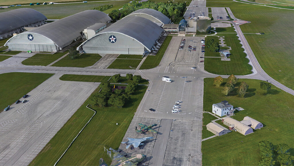
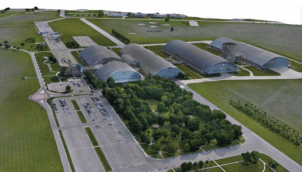
Figure 3: Imagery-based 3D model of the National Museum of the United States Air Force, Dayton, Ohio. Courtesy of Woolpert and the United States Air Force
Download the ASPRS standards document using the following link tinyurl.com/dhp3tert or QR code:

Purchase a printed book of the standards using the following link: tinyurl.com/4radm237.
Acknowledgments
This article will be published concurrently in Photogrammetric Engineering & Remote Sensing and LIDAR Magazine.
The contents of this column reflect the views of the author, who is responsible for the facts and accuracy of the data presented herein. The contents do not necessarily reflect the official views or policies of the American Society for Photogrammetry and Remote Sensing, Woolpert, Inc., NOAA Hydrographic Services Review Panel (HSRP), Penn State, and/or the University of Maryland Baltimore County. 

 Woolpert Vice President and Chief Scientist Qassim Abdullah, PhD, PLS, CP, has more than 45 years of combined industrial, R&D, and academic experience in analytical photogrammetry, digital remote sensing, and civil and surveying engineering. When he’s not presenting at geospatial conferences around the world, Abdullah teaches photogrammetry and remote sensing courses at the University of Maryland and Penn State, authors a monthly column for the ASPRS journal Photogrammetric Engineering & Remote Sensing, sits on NOAA’s Hydrographic Services Review Panel, and mentors R&D activities within Woolpert and around the world. Abdullah is an ASPRS fellow and the recipient of the ASPRS Lifetime Achievement Award and the Fairchild Photogrammetric Award.