Surface-water modeling from lidar-derived DEMs
Over the past 20 years, lidar-derived digital elevation models (DEMs) have become the staple of surface-water hydrography and hydraulic (H&H) modeling. During this same period, lidar has evolved significantly in terms of both absolute three-dimensional (horizontal and vertical) spatial accuracy (<10 cm), and increasing pulse density (>24 pulses per meter square (ppsm)). Most recently, in the commercial lidar market, two distinct lidar technologies have emerged, linear-mode (LM) and Geiger-mode (GM), each with distinct advantages and disadvantages (Lin et al., 2022).
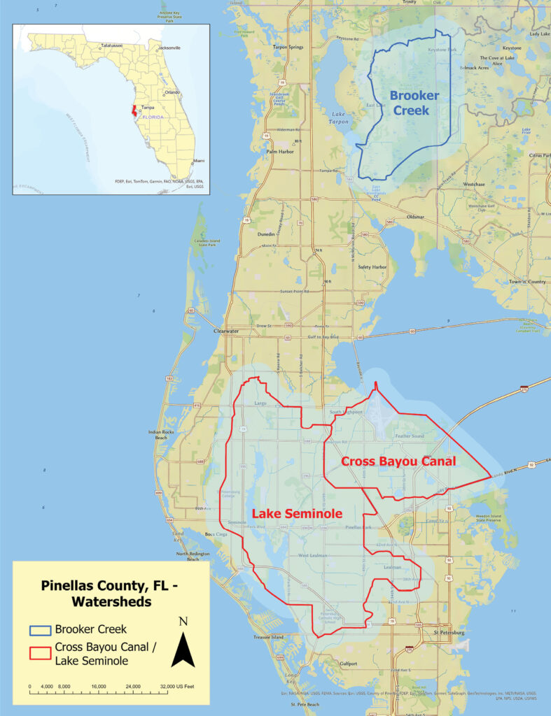
Figure 1: Pinellas County, Florida, showing the northern, mostly undeveloped Brooker Creek watershed and the southern, highly urbanized Cross Bayou Canal/Lake Seminole watershed.
In parallel with the evolution of lidar specifications and technologies, surface-water feature extraction from digital elevation models has also developed. Since the early 2000s the standard methodology for feature extraction involves computing a flow-direction raster and a flow-accumulation raster (Tarboton et al., 1991). While the basic framework has not changed, the methodology for computing these rasters has evolved, from the “D8” method to a multi-directional flow method, to a “D-infinity” method and most recently to a continuous flow At methodology (Ehlschlaeger, 1989). The continuous flow model is currently favored by USGS for the 3D Hydrography Program for the Nation (3DHP FTN)1 for updating the National Hydrography Dataset (NHD) and the Watershed Boundary Dataset (WBD) using USGS 3D Elevation Program (3DEP) products. The current USGS standard for updating the NHD/WBD to 3DHP is to reevaluate on a watershed (Hydrological Unit Code 8) by watershed basis.
Collecting lidar data over entire watersheds can be a costly proposition, so it is difficult to find watersheds that (1) have been maintained over a sufficient time period with little anthropogenic change, and (2) have been surveyed multiple times with differing lidar specifications and technologies. Fortunately, Pinellas County, Florida provides such an opportunity.
The Southwest Florida Water Management District (SWFWMD) houses the Watershed Management Program with responsibilities including stormwater and flood management in the county. Watersheds are reviewed on a rotating five-year maximum interval basis. In the winter of 2007, SWFWMD partnered with the Florida Division of Emergency Management (FDEM) to collect lidar data for the entire county using a Leica ALS40 LM lidar sensor. Then, in 2013, the 2007 lidar data was upgraded to the USGS QL2 standard with some reprocessing and increased breaklining. The county was re-mapped in 2016, with Harris GM technology, and again in 2019, with newer, dual-channel, RIEGL VQ-1560 II LM technology to meet the USGS QL1 and SWFWMD specifications.
As Pinellas County is the most densely populated county in Florida with 3425 people per square mile2, the urbanized areas have remained as highly urbanized areas over the 12-year period and the non-developed areas, designated as nature preserves, have remained as natural areas. For this comparative study, two representative watersheds in Pinellas County were chosen. Cross Bayou Canal/Lake Seminole is typical of urbanized watersheds with a mixture of industrialization and dense population. The terrain includes extensive ditching/berms and infrastructure for stormwater management. Brooker Creek watershed, which stretches across Pinellas and Hillsborough counties (see Figure 1), however, represents “preserved”, more natural portions of the county. The study was restricted to the Pinellas County portion of Brooker Creek, since it has been repeatedly surveyed.
The watersheds
SWFWMD has developed a set of planning units that are used for watershed management and are loosely based on USGS WBD Code 12 HUCs. The SWFWMD planning units, however, also serve as governmental/regulatory units.
For this comparison, two SWFWMD watersheds were chosen to represent the terrain extremes found in the county. The Brooker Creek watershed (Figure 1) encompasses a total of 39.44 square miles (25,645 acres), of which only 17.96 square miles (11,681 acres) are in Pinellas County. This area consists of mostly unaltered terrain with the Brooker Creek Preserve accounting for over 8700 acres surrounded by low-density housing.
The second watershed, in southern Pinellas County, Cross Bayou Canal/Lake Seminole (Figure 1), encompasses 71.75 square miles (45,918 acres) in the most densely populated southern portion of the county. In contrast to Brooker Creek, this watershed is highly urbanized, with extensive ditches, culverts, pipes and other infrastructure systems to protect the dense population from stormwater and flooding.
Digital elevation models
Three lidar-derived DEMs were used for this study. For each, the lidar point cloud and polygonal breaklines (waterbodies over 0.25 acres and double-line drains over 8’ wide) were used to construct a hydro-flattened DEM; single-line drains (SLDs) and/or connectors were not used to hydro-enforce the DEM. DEMs were constructed with 2.5’ x 2.5’ cells and tiled according to the Florida Department of Revenue 5000’ x 5000’ tiling scheme.
USGS/QL2 (2007/2013): constructed from lidar data originally collected in 2007 and reprocessed in 2013. The data was collected at 2 ppsm in 2007 to the USGS QL2 specification, with breaklines approximately to the Lidar Base Specification Version 1.03. The data was then reprocessed by SWFWMD in 2013 with upgraded polygonal breaklines, as described above.
GM (2016): constructed from GM data collected in 2016 by Pinellas County at a pulse density of 20 ppsm with breaklines to meet the SWFWMD polygonal breakline specifications, as described above.
USGS/QL1 (2018). As part of the USGS/FDEM Florida Peninsular Lidar Survey, Pinellas County was remapped in 2018. The data was collected to meet the USGS QL1 specifications (8 ppsm) with USGS Lidar Base Specification v. 2.04 breaklines. SWFWMD upgraded the breaklines to the SWFWMD specifications for polygonal breaklines, as described above, in 2019-20.
Ground-Truth control data
Since 2003, SWFWMD has been using lidar data in support of the Watershed Management Program. In 2007, it started codifying the lidar specifications to support watershed H&H modeling. The SWFWMD Lidar Surveying and Mapping Specification Template 5.2 (9 August 2022: available upon public records request to SWFWMD) includes breakline specifications that are significantly more rigorous than those found in the USGS Lidar Base Specification: (1) all channelized hydrographic features less than 8’ wide are captured as 3D single-line, monotonic drains; (2) all channelized hydrographic features greater than 8’ wide are captured as 3D double-line and polygonal monotonic drains; (3) all waterbodies greater than 0.5 acres are captured as single-elevation 3D features; and (4) all islands over 0.5 acres in waterbodies are captured as 3D single-elevation features. The SWFWMD specifications also include “connectors”—2D features used to maintain surface water connectivity through breach areas. Connectors could include pipes, culverts, and other non-visible breaches. Where breaches occur along double-line drains, two connector lines are used to represent the breach. Where breaches occur along SLDs, one connector line is used to represent the breach.
DEM preprocessing
As the continuous flow At algorithm (Ehlschlaeger, 1989) is a cost-based one, standard practice does not include prefilling the DEM to remove sinks and other artifacts in the surface. Similarly, no smoothing was performed on the hydro-flattened DEMs. Nonetheless, two Esri Arc Hydro tools for DEM manipulation were used to preprocess each DEM:
To ensure that artificial path connections through waterbodies maintain a valence no greater than three, the double-line drains (polygons) were merged with the waterbody polygons and the Burn Flat Polygons into DEM tool in Arc Hydro was used to re-enforce these areas into the DEM.
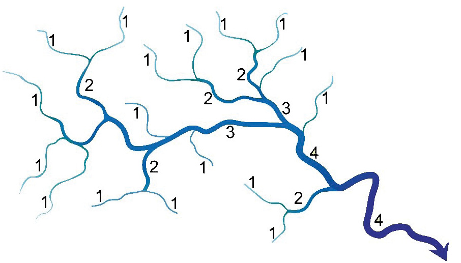
Figure 2: Strahler (1952) stream ordering hierarchy where the smaller streams (order 1) flow into consecutively larger (order 2) streams, and so on.
Where the connectors, i.e. breaches or culverts, were represented as paired linear features, one of the pairs was removed, the remaining member repositioned to the center of the breach/culvert, and the single-line connectors were enforced into the DEM using the Burn Lines into DEM tool.
Analytical processing
With the possible exception of USGS/NHD artificial paths (through waterbodies), the SWFWMD SLDs represent the channelized hydrological features under 8’ wide and should agree closely with the channelized features identified for the 3DHP update for the NHD. For this comparison, Esri ArcGIS Pro was used to buffer the SLDs by 5’ and the resulting polygons were used to select the results of the flowlines modeled from each of the three DEMs. The linear distance of SWFWMD SLDs, the ground-truth, and the elevation-derived hydrography (EDH), i.e. the modeled channel, were then used to determine the degree of agreement between SWFWMD ground-truth and the modeled EDH results.
Two levels of analysis were performed to help evaluate the differences between the lidar-derived DEMs. Firstly, the lengths of each Strahler stream order were computed and compared to each other, exclusive of the SWFWMD ground-truth. The goal was to determine the extent of agreement among the lidar-derived DEMs for Strahler orders 1–4. The second analysis entailed using ArcGIS Pro to “select” the stream network as derived from each DEM for comparison to the SWFWMD ground-truth network.
3DHP modeling approach
An ArcGIS Pro workflow focusing on the continuous flow At algorithm was developed. The Derive Continuous Flow (Spatial Analyst) tool was used to construct the flow-direction and flow-accumulation rasters from each of the three DEMs. The stream raster network was derived from these rasters using a flow accumulation of 6 acres (261,360 square feet) and specifying Strahler stream ordering (see Figure 2; Strahler, 1952) using the Derive Stream as Raster tool. The stream raster network was vectorized using the Stream to Feature tool and the flow-direction raster that was previously generated (Figure 3).
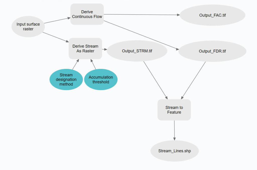
Figure 3: Esri ArcGIS Pro ModelBuilder schematic for continuous flow At 3DHP workflow.
Results and discussion
The analysis of the resulting flowline networks focused on two aspects: (1) the numbers and lengths of Strahler order 1–3 reaches (see Figure 2), as these represent the SLDs and channels that would be represented in the EDH updates, and (2) the agreement between the modeled flowline networks and the SWFWMD ground-truth.
Flowline network composition (number and length)
As expected, the flowline network composition was similar for each DEM-type for both watersheds. In the non-disturbed Brooker Creek watershed, there was a slight tendency for more flowlines to be observed in Strahler orders 1–3 from the GM-derived DEM relative to either of the LM-derived DEMs (Table 1). However, the total number of linear miles of reaches modeled is slightly larger from the QL1 LM-derived DEM, 219.6 miles, than from the QL2 LM- or GM-derived DEMs, 195.1 and 213.0 miles respectively.
Curiously, although the network composition metrics for the small, Strahler order 1 reaches, i.e., those that are below the USGS/EDH length threshold (50 m; 164’), totaled approximately the same length among the DEMs (~1.1 miles), the QL1-derived DEM resulted in 26% fewer flowlines than the QL2-derived flowlines and almost 20% fewer lines than the GM-derived flowlines. Nevertheless, although the average length of the flowlines modeled from QL1-derived DEMs was larger than either the QL2- or GM-derived DEMs, the difference between any was not significant (F2,235 = 0.96, p = 0.38).
In Cross Bayou Canal/Lake Seminole too, the three lidar-derived DEMs produced similar network metrics for Strahler orders 1-3, with the USGS/QL1 DEM resulting in the longest flowline network: 718.1 miles compared to 702.6 miles and 706.9 miles for the QL2 and GM-derived flowline networks respectively (Table 2). Again, the slight differences in combined flowline length cannot be attributed to the difference of the lidar-derived DEMs.
In this urbanized watershed, however, the between-DEM variance for stream length in the small Strahler order 1 flowlines less than 50 m is significantly different (F2,1022 = 5.15, p = 0.005), indicating that the length of the small upper reaches is dependent on the original DEM used for the modeling, the LM-derived DEMs yielding longer upper-level reaches than the GM-derived DEM.
Flowline network geometry
While the flowline network composition metrics do not show significant differences that could be attributed to the underlying DEMs, their spatial geometries, especially in wetlands, are considerably different. As an example, in the Brooker Creek watershed, the three DEMs produced completely different paths through wetland areas (Figure 4).
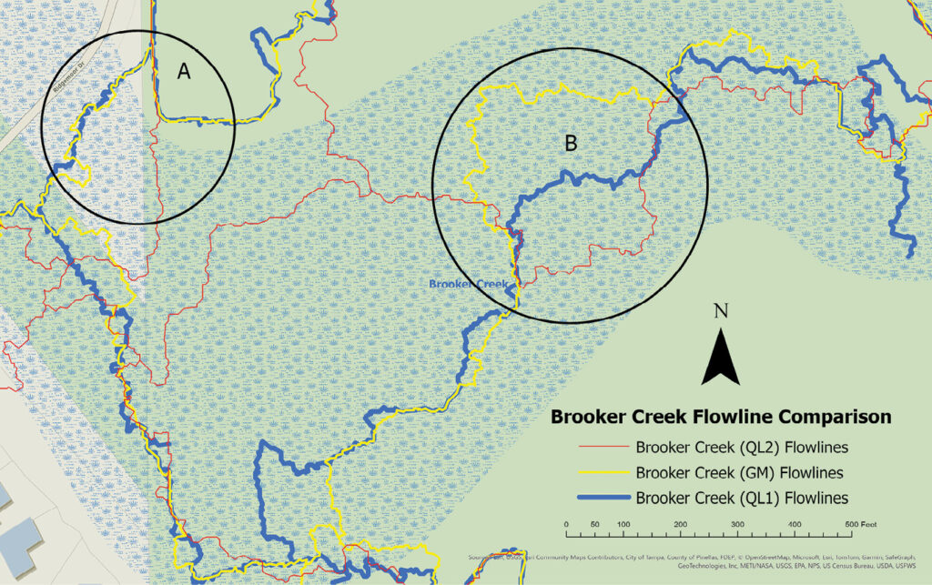
Figure 4: Comparison of flowlines in wetlands at Brooker Creek Preserve, derived from continuous flow. modeling: (A) area of close similarity between the QL1- and GM-derived flowlines; (B) area of divergence between the three DEM-types.
In the more urbanized Cross Bayou Canal/Lake Seminole watershed, there are also areas where the flowlines are in close agreement among all three DEM-types (Figure 5A), as well as areas where there is little agreement (Figure 5B). In the urban areas, there were several areas where the GM-derived DEM resulted in flowlines that stopped, whereas the QL1 lidar-derived DEMs provided continuity (Figure 5C).
Comparison to SWFWMD ground-truth
As indicated previously, the SWFWMD lidar specification prescribes that all channelized features are captured as either single-line (less than 8’ wide) or double-line (greater than 8’ wide) drains. The SLDs in the watersheds were buffered to produce polygons and used to clip the flowlines resulting from each of the three DEM-types. The total lengths of the clipped lines were summarized (Tables 3 and 4) to indicate the degree of agreement between flowlines and the ground-truth for each DEM-type. In both watersheds, there was over 93% agreement between the QL1 LM-derived flowlines and the SWFWMD ground-truth. The GM-derived DEM performed slightly better in the Brooker Creek watershed (92.6% agreement) than it did in the Cross Bayou Canal/Lake Seminole watershed (81.4% agreement). Both the QL1- and GM-derived DEMs performed better in both watersheds than the QL2-derived DEM.
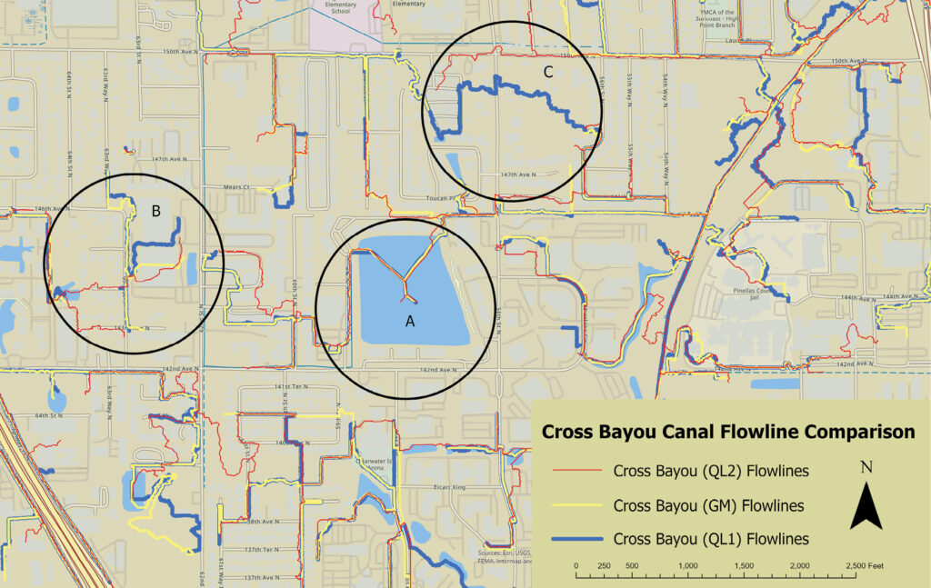
Figure 5: Comparison of flowlines at Cross Bayou Canal/Lake Seminole, derived from continuous flow modeling: (A) – area of close similarity between the QL1- and GM-derived flowlines; (B) – area of divergence between the three DEM-types; and (C) – area where QL1 lidar-derived DEMs resulted in continuous flow paths; there are other similar areas in the watershed.
Parting comments
The British statistician, George Box, is frequently noted for saying that, “All models are wrong, some are useful” (Box and Draper, 2007, 414). While Box was talking about statistical models, the same could easily be applied to DEMs. We always need to remember that the DEM is a model of the earth, and that the results are further abstracted as a result of the continuous flow At model used to produce the flowlines. With that caveat and with respect to using lidar-derived DEMs for EDH for these two watersheds, therefore, we conclude:
Small upper reaches, under the EDH threshold, were equally well resolved in the non-urbanized watershed (Brooker Creek), but in the urban environment (Cross Bayou Canal/Lake Seminole), both LM-derived DEMs resolved significantly more flowlines. This may have resulted from the algorithms used by the lidar providers to decimate the GM lidar. The decimation or smoothing had little effect in the rural terrain, where the LM lidar also produced a smoother DEM. In the urban terrain, however, the LM lidar point clouds were more detailed and provided additional definition for those upper reaches.
In terms of total network length and reach-number metrics, each of the DEMs performed well, and the metrics were not significantly different. But in both watersheds, the QL1-derived DEMs produced slightly more reaches and a slightly longer network.
Geometric differences that could be attributed to the DEM were most striking when the flowlines were compared to SWFWMD ground-truth. In both watersheds, the QL1-derived DEMs produced a geometric network that more closely resembled the ground-truth. Again, possibly as a result of the decimation algorithm used for the GM lidar, the QL1 advantage was greater in the urban watershed (93.6% vs. 81.4% agreement) than in the rural watershed (93.4% vs. 92.6%).
Overall, both the QL1 and GM high-density lidar-derived DEMs outperformed the lower-density QL2-derived DEM for EDH extraction. Future comparisons between the high-density technologies need to account for GM decimation and other low-level lidar processing differences, such as DEM construction methodologies and hydro-conditioning techniques.
Alvan “Al” Karlin, PhD, CMS-L, GISP is a senior geospatial scientist at Dewberry, formerly from the Southwest Florida Water Management District (SWFWMD), where he managed all the remote sensing and lidar-related projects in mapping and GIS. With Dewberry, he serves as a consultant on Florida-related lidar, topography, hydrology, and imagery projects, as well as general GIS-related projects. He has a PhD in computational theoretical genetics from Miami University in Ohio. He is vice president of ASPRS, a director of the ASPRS Florida Region, an ASPRS Certified Mapping Scientist-Lidar, and a GIS Certification Institute Professional.
References
Box, G.E.P. and N. R. Draper, 2007. Response Surfaces, Mixtures, and Ridge Analyses, 2nd edition, John Wiley & Sons, Hoboken, New Jersey, 880 pp.
Ehlschlaeger, C. R., 1989. Using the AT search algorithm to develop hydrologic models from digital elevation data, International Geographic Information Systems (IGIS) Symposium, 89: 275-281.
Lin, Y-C., S. Jinyuan, S-Y. Shin, Z. Saka, M. Joseph, R. Manish, S. Fei, and A. Habib, 2022. Comparative analysis of multi-platform, multi-resolution, multi-temporal lidar data for forest inventory, Remote Sensing, 14: 649-676.
Strahler, A.N., 1952. Dynamic basis of geomorphology, Geological Society of America Bulletin, 63: 923-938.
Tarboton, D. G., R. L. Bras, and I. Rodriguez–Iturbe, 1991. On the extraction of channel networks from digital elevation data, Hydrological Processes, 5: 81–100.
1 3dhp-for-the-nation-nsgic.hub.arcgis.com/
2 pinellas.gov/about-pinellas-facts/
3 pubs.usgs.gov/tm/11b4/Version1.0/TM11-B4.pdf
4 usgs.gov/media/files/lidar-base-specification-v-20