This highlight article was inspired by a comment I received from Richard C. Maher, PLS, president of KDM Meridian:
“I attended both of your American Society for Photogrammetry and Remote Sensing (ASPRS) workshops during Geo Week 2024 in Denver. Even after 24 years as a land surveyor, I can still use refreshing on how to explain the basics to my clients and surveyors-in-training. Your in-depth discussion on the difference between the standard deviation and the root mean square error (RMSE) was very appreciated. I also appreciated the concepts of the true datum and the survey (pseudo) datum you introduced. As one who loves to test and prove that our equipment can rarely do better than the specifications, I’ll say unequivocally that surveyors using real-time kinematic (RTK) positioning are far too optimistic about their true accuracy and commonly don’t understand apparent relative accuracy due to a fundamental misunderstanding of the error sources different between GPS and conventional measurements. The nature of random error in GPS follows a different stochastic model than conventional instrumentation. If surveyors simply employed the same checking standards and methods you prescribe in the ASPRS specifications, they’d stop telling me how well their GPS did under a canopy, or how they can get “hundredths.” My intention isn’t to make their work more difficult but to ensure that our methods are rigorous and reliable… I’m interested in seeing your future appendix that talks about suggested survey accuracies when not provided by surveyors. Due to the importance of these topics to the thousands of practicing surveyors in the nation who could not attend Geo Week, could you please shed light on the concepts you presented in Denver regarding surveying and mapping accuracy and the role of the correct understanding of the datum?”
In my response to this request, I will address these important issues in separate sections.
Standard deviation versus root mean square error (RMSE) estimation
Before we discuss the difference between standard deviation and RMSE as accuracy measures, let us elaborate on the statistical meaning of each.
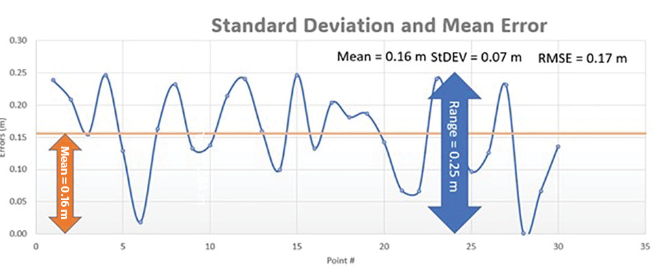
Figure 1: Standard deviation measures the error fluctuation around a mean value of 0.17 m.
Standard deviation is a statistical measure of the fluctuation or dispersion of individual errors around the mean value of all the errors in a dataset. Figure 1 illustrates how the errors fluctuate around a mean error value of 0.16 m. This fluctuation is represented by the standard deviation value, or 0.07 m.
The standard deviation is calculated as the square root of variance by determining each error’s deviation relative to the mean as given in the following equation:

where: x is the mean error in the specified direction, xi is the ith error in the specified direction, n is the number of checkpoints tested, i is an integer ranging from 1 to n. |
RMSE is the square root of the average of the set of squared differences between dataset coordinate values and coordinate values from an independent source of higher accuracy for identical points. It is obvious from this definition that RMSE differs from standard deviation by the magnitude of the mean error existing in the data. This becomes clear from the difference between the previous equation, defining the standard deviation, and the following RMSE:

where: xi(map) is the coordinate in the specified direction of the ith checkpoint in the dataset, xi(surveyed) is the coordinate in the specified direction of the ith checkpoint in the independent source of higher accuracy, n is the number of checkpoints tested, i is an integer ranging from 1 to n. |
When RMSE is computed, we do not subtract the mean checkpoint error, so RMSE represents the full spectrum of the error found in a checkpoint, including the mean error, whereas, in computing the standard deviation, we subtract the mean error from every checkpoint error, making it a measure of the fluctuation of individual errors around the mean value of all the errors. This RMSE characteristic makes it useful in flagging biases in data, as it provides an early warning system for the technician that the standard deviation fails to do.
Biases and systematic errors in data
Now we understand the difference between the standard deviation and RMSE, let us see how such favoring of the RMSE helps the geospatial mapping production process and validation of the accuracy of its products. Geospatial mapping products are subject to systematic errors or biases from a variety of sources. These biases can be caused by things like using the wrong version of a datum during the product production process, or using the wrong instrument height for the tripod during the survey computations for the ground control points or the checkpoints. There are other sources of biases that can be introduced during the production process. For instance, using the wrong elevation values in digital elevation data can result in biases during the orthorectification process, and using the wrong camera parameters (such as focal length) or the wrong lens distortion model can lead to biases in the final mapping product.
Systematic error can cause the product to fall below acceptable project accuracy levels. Thankfully, provided the appropriate methodologies are applied, systematic error can be identified, modeled, and removed from the data. This is not the case with random error: even if we discover it, we cannot eliminate it. However, we can minimize random error magnitude through adherence to a stringent production process, adopting sound quality control practices, or the use of more accurate instruments. To illustrate systematic errors or biases in data, we will evaluate the scoreboards of four archers who vary in their aiming skills, illustrated in Figure 2.
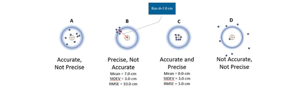
Figure 2: Scoreboards for four archers with varied aiming skills.
For Board A, the archer landed the arrows around the bullseye, but the shots are scattered spatially around the center point. By contrast, Board B reflects good spatial clustering, but the shots are clustered around a point far away from the bullseye. Board C is what one wants accuracy to be, with all shots clustered at the aimed spot. Board D demonstrates extremely undesirable results, possessing neither good clustering, nor good aiming.
When we measure accuracy, results like boards B and C are the most desirable. Board C should be preferred, as it represents clean results: All shots are at the bullseye. We can describe archer C as “accurate and precise.” Although archer B’s results lack good aim, the shots are clustered well. We describe archer B as “precise but not accurate.” Even though archer B is not accurate, why are these results still acceptable? Examine the scoreboard for archer B again: if we shift the locations of all the clustered arrows by a fixed distance d, or 7.0 cm, the results will match the results from archer C. This distance d or 7.0 cm represents the systematic error; once it is corrected, the final accuracy will be satisfactory.
But why did such a precise archer miss the bullseye to begin with? We must consider what may have taken place at the archery range to cause archer B to miss. Perhaps the archer was using a sight scope hooked to the archer bow. Having all the arrows land in a tight cluster away from the bullseye is a strong indication of a mechanical failure of the sight scope that caused the arrows to go to the wrong place. Once archer B’s sight scope is properly calibrated, the archer scoreboard in the second archery session will look just like archer C’s board. The same logic can be applied to geospatial products such as lidar point clouds or orthoimagery. That is why it is crucial to use accurate checkpoints when verifying product accuracy. These checkpoints will help us quantify any existing systematic errors, allowing us to remove this error from the data in the same way that properly calibrating archer B’s sight scope corrects the archer future shots.
True datum versus surveying pseudo datum
When we conduct field surveying, we are trying to determine terrain positions and shapes with reference to a specific geodetic datum. According to the U.S. National Geodetic Survey (NGS), a geodetic datum is defined as “an abstract coordinate system with a reference surface (such as sea level, as a vertical datum) that serves to provide known locations to begin surveys and create maps.” Because our surveying techniques, and therefore our mapping techniques, are not perfect, our surveying techniques provide only approximate positions that put us close to the true, datum-derived positions (Figure 3). When we use an inaccurately surveyed network to control another process such as aerial triangulation, we are fitting the aerial triangulation solution to an observed datum. The degree of approximation depends on the accuracy of the surveying technique or technology employed in that survey. The RTK field surveying technique, for example, can produce positions that are accurate to 2 cm horizontally and perhaps 2-3 cm vertically. The differential leveling technique used to determine height can produce elevations that are accurate to the sub-centimeter. The lesson to learn here is that our surveying techniques, no matter how accurate, do not represent the true datum—but they can get us close to it.

Figure 3: Datums and error propagation in geospatial data.
Surveying and survey (pseudo) datum
When we task surveyors to survey the ground control network with reference to a certain datum, usually a true datum such as NAD83 or WGS84, they can determine the positions of the control network to that datum only as close as the surveying techniques allow. In other words, the coordinates used to control the mapping process represent an observed or survey datum that forms a pseudo datum, green mesh in Figure 3, but not the original intended or true datum represented by the solid green in Figure 3. For example, if we are trying to determine point coordinates in NAD83(2011), the surveyed coordinates used in aerial triangulation or lidar calibration represent a datum that is close to NAD83(2011) but not exactly NAD83(2011), due to the inaccuracy in our surveying techniques. That inaccurate survey represents a survey datum. Besides the inaccuracy in the surveying techniques, another layer of errors (i.e., distortion) could be added to the surveyed coordinates when we convert geographic positions (in latitude and longitude) to projected coordinates or grid coordinates, such as state plane coordinate systems.
Mapping to the mapping datum
Any mapping process we conduct today inherits two modeling errors that influence product accuracy. The first modeling error is caused by the inaccuracy of the internal geometric determination during the aerial triangulation, or the boresight calibration in the case of lidar processing. The second modeling error is introduced by the auxiliary systems, such as GNSS and IMU, and has inherent errors caused by the survey datum. Therefore, when we use mapping products to extract location information, we are determining these locations with reference to the survey or pseudo datum and not the true intended datum. The point coordinates for NAD83(2011) are determined not according to the survey datum of the ground control network but through a new reality of mapping datum. The mapping datum, represented with the blue mesh in Figure 3, inherits the errors of the survey datum, which were caused by the inaccuracy of our surveying techniques and the errors caused by our mapping processes and techniques.
Correct approach to accuracy computation
To reference the accuracy of determining a mapped object location within a mapping product with reference to the original intended datum such as NAD83(2011), we need to examine the layers of error that were introduced during the ground surveying and mapping processes (Figure 3).
Currently, users of geospatial data express product accuracy based on the agreement or disagreement of the tested product with respect to the surveyed checkpoints, ignoring checkpoint or ground control errors that have resulted from inaccurate surveying techniques. In other words, users consider the surveyed points to be free of error. The following section details how errors are propagated into the mapping product when we are trying to determine the location of a ground point “A”. Let us introduce the following terms—refer to Figure 3 for localizing such error terms:
ACCSurveyDatum equals the accuracy in determining the survey datum, generated when realizing the intended or true datum through surveying techniques. In other words, it represents the errors in the surveyed checkpoints. Due to this inaccuracy, the point will be located at location A.. (Figure 4).
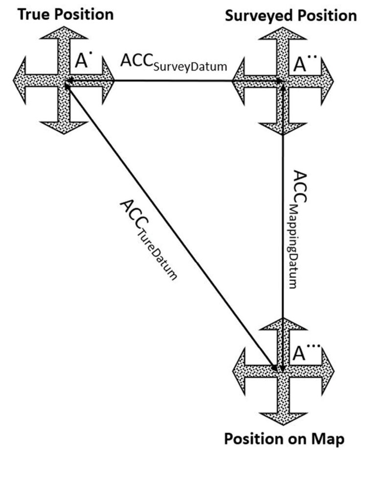
Figure 4: Influence of error propagation on point location accuracy.
ACCMappingDatum equals the accuracy of determining the mapping datum, or the errors introduced during the mapping process, with reference to the already inaccurate survey datum represented by the surveyed checkpoints. In other words, it is the fit of the aerial triangulation (for imagery) or the boresight/calibration (for lidar) to the surveyed ground control points represented as the survey datum. This accuracy is measured using the surveyed checkpoints during the product accuracy verification process. Due to this inaccuracy, the point will be located at location A… (Figure 4).
ACCTrueDatum equals the accuracy of the mapping product with reference to the true datum, for example NAD83(2011). The point location A. (Figure 4) is considered the most accurate location determined with reference to the true datum.
Using the above definitions, the correct product accuracy should be modeled using error propagation principles according to the following formula:
 |
However, according to our current practices, product accuracy is computed according to the following formula, ignoring errors in the surveying techniques:
 |
More details and examples on the suggested approach can be found in my published article1 on the topic and Edition 2 of the ASPRS Positional Accuracy Standards for Digital Geospatial Data2.
The new approach to computing map accuracy
According to this new approach to computing map accuracy and since we are dealing with three-dimensional error components, we would need to employ vector algebra to accurately compute the cumulative error.
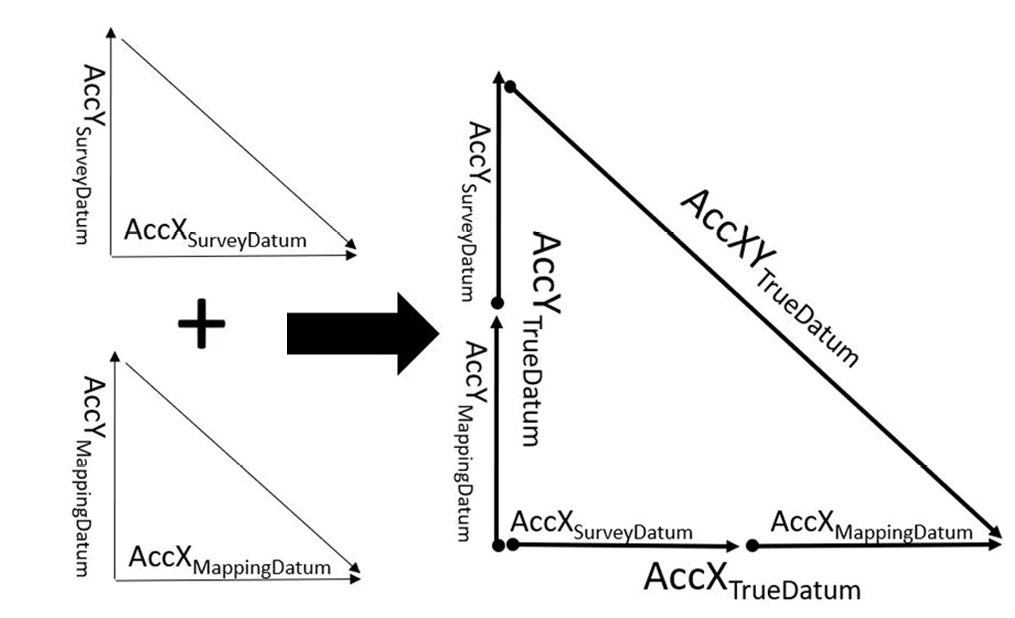
Figure 5: Vector representations of error components.
Computing horizontal accuracy
To compute the horizontal accuracy for a two-dimensional map, as with orthorectified imagery, we will ignore the error component of the height survey. In other words, we will use the error component from easting and northing only. We will also assume that the accuracy of determining the X coordinates (or eastings) is equal to the accuracy of determining the Y coordinates (or northings). Using error propagation principles and Euclidean vectors in Figures 4 and 5, we can derive the following values for product horizontal accuracy:
 |
 |
 |
As an example, when modeling horizontal product accuracy according to the above formulas, let us assume the following:
- We are evaluating the horizontal accuracy for orthoimagery using independent checkpoints.
- The control survey report states that the survey for the checkpoints, which was conducted using RTK techniques, resulted in accuracy of RMSEXorY equal to 2 cm.
- When the checkpoints were used to verify the horizontal accuracy of the orthoimagery, the result was an accuracy of RMSEXorY equal to 3 cm.
Thus, from equations 3, 4 and 5:
 |
![]()
 |
EQ |
 |
E |
The value of 5.1 cm is the true accuracy of the product versus the following value of 4.24 cm used commonly today that ignores the errors introduced during the ground surveying process:
 |
E |
Computing vertical accuracy
Similarly, for vertical accuracy determination of elevation data derived from lidar or photogrammetric methods, we need to consider the error in the surveyed elevation as an important component.
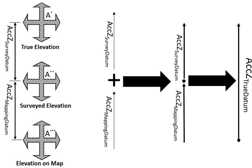
Figure 6: Influence of error propagation on point elevation accuracy.
Using error propagation principles and the Euclidean vectors of Figure 6, we can derive the following value for vertical product accuracy:
 |
E |
As an example, when modeling vertical product accuracy according to the above formulas, let us assume that:
- We are evaluating the vertical accuracy for a mobile lidar dataset using independent checkpoints.
- The control survey report states that the survey of the checkpoints, which was conducted using RTK techniques, resulted in an accuracy of RMSEZ equal to 3 cm.
- When the checkpoints were used to verify the vertical accuracy of the lidar data, the results was an accuracy of RMSEZ equal to 1 cm.
Thus, from equation 6:
 |
EQ |
The value of 3.16 cm is the true vertical accuracy of the lidar dataset, versus the value of 1 cm derived by the mapping technique used commonly that ignores the errors introduced during the ground surveying process.
The role of RMSE in revealing biases in data
Now, let’s see how we are going to assess the accuracy computations, and whether we can spot problems in the data. We assume a scenario in which systematic error was introduced into a lidar dataset during the product generation. Say a technician used the wrong version of the geoid model when converting the ellipsoidal heights of the point cloud to orthometric heights, which caused a systematic error or bias of 0.16 m in the computed elevation of the processed lidar point cloud. Table 1 lists the results of the accuracy assessment where 30 checkpoints are used for the test.
To analyze the accuracy results, first look at the error mean value in Table 1. (See PDF for Tables) We clearly notice that the mean error is high as compared to the RMSE and the standard deviation. The ASPRS Positional Accuracy Standards for Digital Geospatial Data advise that a mean error value that is more than 25% of the RMSE is an indication of biases in the data that need to be dealt with and resolved before accepting and delivering the lidar data. So, we will focus on the results in Table 1 for further analysis. A high mean error value is a good indication that biases are present in the data, but we need to further investigate how high the mean value is compared to RMSE and standard deviation. Slight differences between these statistical measures’ values are acceptable. Looking at the results of Table 1, the mean error reaches 91% of the RMSE value, which is not acceptable according to the ASPRS standards. We also need to compare the RMSE to the standard deviation. Note that they are 0.170 m and 0.069 m, respectively. An RMSE value more than twice the standard deviation is a strong indication that biases may be present in the data. Remember that, in the absence of systematic errors, i.e., biases, the RMSE and the standard deviation should be equal. This conclusion is also supported by the fact that the mean is twice as high as the standard deviation.
Now that we have concluded that the data has biases in it, let us see how we will remove these without reproducing the product from scratch. For lidar data, we will need to raise or lower the computed heights for the point cloud by the amount of the bias—in this case, 0.16 m. Since the mean is a positive value, and the values in the “Error Values” column were computed by subtracting the lidar elevation from the checkpoint elevation, or:
Error = Surveyed Elevation – Lidar Elevation |
We can then conclude that the terrain elevation as determined from the lidar data is lower than that measured by the surveyed checkpoints. Thus, we need to raise the lidar elevations by 0.16 m. Table 2 illustrates the bias treatment we introduced above, where the modified accuracy assessment values are listed in column “Unbiased Error Values.” All we did here was raise, or z-bump, the elevations of the point cloud by the amount of the bias, 0.16 m.
Similarly, if such an analysis were conducted to investigate the horizontal positional accuracy of an orthoimage, all we would need to do is modify the coordinates of the tile’s header by the amount of the calculated biases without the need to reproduce the orthoimages. It is worth mentioning that removing the bias based on the “mean” value will not necessarily reduce the value of the RMSE by the same amount, as the degree of improvement in the recalculated RMSE value depends on the value of the standard deviation. For datasets with low standard deviation value and low rates of fluctuation, removal of the biases will improve the RMSE by a more significant degree. With the data cleaned from the bias effect, all conditions for good accuracy results are satisfied and clearly presented in Table 2. The mean error is zero as the bias was removed, and the standard deviation and the RMSE values are equal.
The new approach and challenges for users
As we introduced the new approach in modeling products’ accuracy, I was surprised by the following findings.
Survey accuracy and surveyors’ awareness
As expressed in equation 1, the new approach requires the user to enter an absolute accuracy figure for the surveyed local network. To my surprise, I found most surveyors I spoke with were either not aware of where to find this accuracy figure in the instrument processing report, or blindly trusted numbers in reports where the accuracy is presented as a quality measure that does not relate to the absolute accuracy as called for by the new approach. I reviewed several processing reports from some surveying instruments where such a figure approaches zero, for example 0.002 m.
Surveying instruments manufacturers and survey accuracy
To follow up on this, the ASPRS accuracy standard working group contacted several manufacturers of surveying instruments, but we did not get straight answers to our request as most manufacturers do not report such absolute accuracy figures. To me, it seems that a reported accuracy figure of close to zero represents a precision measure from multiple survey sessions of the same point. Users of these instruments need to know that all current surveying instruments, no matter how accurate, cannot produce a surveying accuracy of 0.002 m.
Surveyors’ and mappers’ power
Surveyors and other users of these instruments need to unite and exert their efforts with the surveying equipment manufacturers to provide access to the absolute accuracy of the network survey. Without it, we cannot comply with the accuracy assessment method dictated by the new ASPRS standards. For the time being, and until manufacturers provide us with this accuracy, Table 3—which we included in the forthcoming version of the ASPRS Positional Accuracy Standards for Digital Geospatial Data —can be used for the default accuracy values in situations where the survey accuracy is not available or known.
The need to revise the professional practice certification programs
The issues raised in this article are a clear indication of the lack of awareness among professionals about the very issue impacting basic surveying and mapping practices. I call on all professional societies such as NSPS, ASPRS, ASCE, TRB, and others to lead an awareness campaign to educate their members on the importance of this issue. The time is right to start this campaign as we head toward an entire National Spatial Reference System (NSRS) modernization program, to which NOAA and NGS are leading us. The new North American Terrestrial Reference Frame of 2022 (NATRF2022) and the North American-Pacific Geopotential Datum of 2022 (NAPGD2022) will offer more accurate and evolving horizontal and vertical datums, which makes the issues raised in this article even more crucial to the success of our business. Similarly, I put forward a call to all state agencies—which are tasked with the professional certification of surveyors, mappers, and engineers—and NCEES to revise their certification testing materials to include topics raised in this article. Without doing this, we risk the health, safety, and welfare of the public. 
Note: This article is running in both Photogrammetric Engineering & Remote Sensing and LIDAR Magazine.
 Woolpert Vice President and Chief Scientist Qassim Abdullah, PhD, PLS, CP, has more than 45 years of combined industrial, R&D, and academic experience in analytical photogrammetry, digital remote sensing, and civil and surveying engineering. When he’s not presenting at geospatial conferences around the world, Abdullah teaches photogrammetry and remote sensing courses at the University of Maryland and Penn State, authors a monthly column for the ASPRS journal Photogrammetric Engineering & Remote Sensing, sits on NOAA’s Hydrographic Services Review Panel, and mentors R&D activities within Woolpert and around the world.
1 Abdullah, Q., 2020. Rethinking error estimations in geospatial data: the correct way to determine product accuracy, Photogrammetric Engineering & Remote Sensing, 86 (7): 397-403, July 2020.