Note: This is a slightly shortened version of the published paper by the same authors, which is listed as the third reference in the bibliography at the end of the article.
Introduction
Originally, photogrammetry and laser scanning developed as competing disciplines, providing specific advantages and using individual processing pipelines while aiming at the airborne collection of 3D point clouds. As an example, lidar sensors measure multiple responses of the reflected signal, which is advantageous to measure both on and below vegetation. On the other hand, georeferencing accuracy is basically defined by the accuracy of the trajectory as measured by an integrated GNSS/IMU system. In combination with the accuracy of lidar range measurement of about one centimetre, this limits the accuracy of lidar point clouds captured from a moving platform to a few centimetres. In contrast, Multi-View-Stereo-Matching (MVS) of overlapping images potentially provides point cloud accuracies that directly correspond to the ground sampling distance (GSD) of the imagery. Thus, a proper selection of the captured image scale enables direct control of geometric accuracies. However, this presumes suitable redundancy during image matching, which can be hindered, for example, by occlusions or texture-less images in certain scenarios. In order to benefit from the respective advantages, systems for joint collection and evaluation of lidar and image data are becoming commonplace. This allows for applications like the collection of UAV point clouds at millimeter accuracy, which have not been possible so far. We demonstrate this high-accuracy data collection in the context of a project for the deformation monitoring of a ship lock due to geological subsidence.
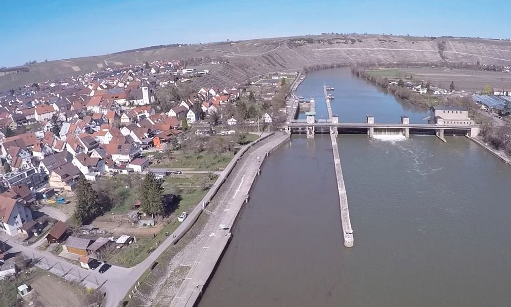
Figure 1: Test area with the village of Hessigheim and the ship lock area.
Figure 1 depicts our test site, which includes a ship lock and its facilities, the river Neckar and the riparian area as well as vegetated areas, farmland, and residential areas of the surrounding village of Hessigheim, Germany. In this area, geological subsidence results in local displacements of about 6-10 mm/year. These changes are monitored by terrestrial data collection twice a year using geodetic instruments such as levels, total stations and differential GNSS (Kauther and Schulze, 2015). This was the reason to establish a network of pillars and marked points for signalization. However, economic reasons limit these engineering geodesy techniques to measures at specific parts of built structures or natural objects. In contrast, airborne platforms allow for area-covering 3D measurement. Since photogrammetric data collection at millimeter scale requires imagery at a similar resolution, this requires the low flying altitudes that are feasible with UAV platforms. If signalized control points are additionally available, photogrammetric image processing can meet such accuracy specifications. However, our project aims at the measurement of subsidence of terrain surfaces, which are covered to a considerable extent by vegetation such as trees, bushes and shrubs. This motivated the additional use of lidar due to its ability to penetrate such vegetation. The point cloud of our test area is depicted in Figure 2, with color coding representing the number of reflections of the respective lidar pulse. Such multiple returns are measured and analyzed during full-waveform recording. Furthermore, the labels represent the IDs of the signalized points available in the test area. While this network was originally established during terrestrial monitoring, it is also applied during our accuracy investigations of UAV-based data collection. Clearly, these signals are rather dense in the ship lock area, which is the main object of interest.
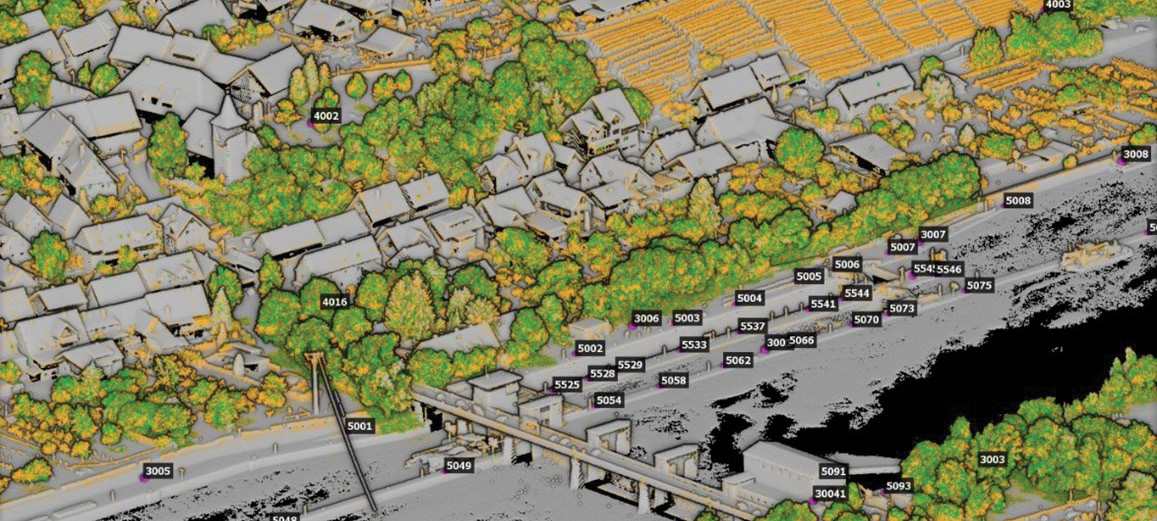
Figure 2: Lidar point cloud captured at the ship lock area with color coding representing the number of returns and labels displaying IDs of signalized targets.
For deformation monitoring, multiple UAV flights were captured for a period of three years. Joint orientation of laser scans and images in a hybrid adjustment framework then enabled 3D point accuracies at millimeter level. This process integrates photogrammetric bundle block adjustment with direct georeferencing of lidar point clouds and thus improves georeferencing accuracy for the lidar point cloud by an order of magnitude.
Test set-up and data collection
Figure 3 depicts the planned flight configuration for our test area. The ortho image depicts our area of interest, which features a maximum site extension of 570 m (east-west) x 780 m (north-south). In addition to the respective lidar strips, which are coloured individually, the figure includes the distribution of the signalized ground points already shown in Figure 2.
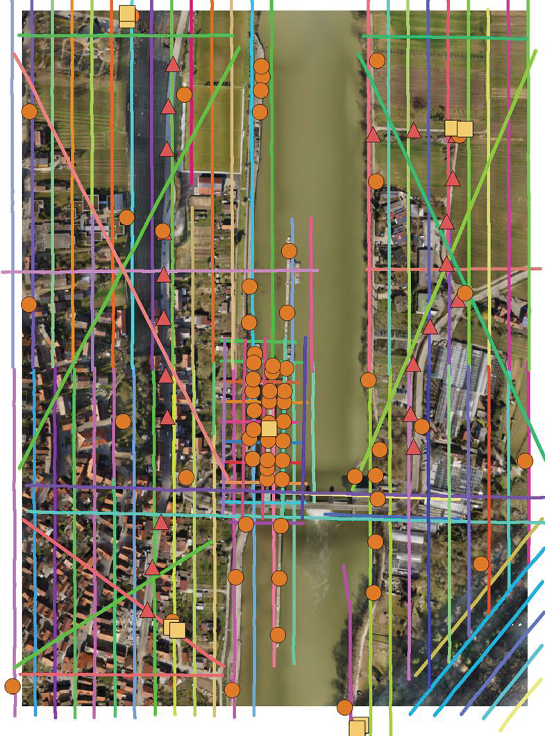
Figure 3: Area of investigation with captured lidar strips (colored individually), lidar control planes (dark yellow squares), checkerboard targets (orange dots) and non-signalized height check points (red triangles).
In Figure 3, so-called photogrammetric control planes (PCP) are represented by orange circles. Figure 4 (left) gives an example of such a checkerboard signal. These targets were scattered within the test area and served as control or check points during automatic aerial triangulation (AAT) of the imagery. In our test area the checkerboards were mounted on pillars, tripods, and directly on the ground. They have a diameter of 27 cm in order to enable automatic measurement of corresponding image coordinates. Figure 4 (right) depicts a so-called lidar control plane (LCP). These signals, represented by dark yellow squares in Figure 3, are constructed by two roof-like oriented planes with each roof plane featuring a size of 40 cm x 80 cm. Thus they consist of distinct planar geometries with known position and orientation in space. Their inclination of 45° provides both a vertical and a horizontal component to be analyzed during accuracy investigations on lidar point georeferencing. In contrast, the horizontal PCPs only contribute a vertical component. The accuracy of both PCP and LCP coordinates allows their use as either control or check points during our investigations. In contrast, the points represented as red triangles in Figure 3 were just marked on the street and used as additional height check points since their positional accuracy is insufficient for the aspired accuracy level. Point coordinates for the respective signals were provided by geodetic survey, i.e. either GNSS or tacheometric measurement. The accuracy of these reference points is in the range of 1-3 mm. Providing such quality for a considerable number of points scattered in a larger test area requires great effort, while the inevitable remaining errors may already influence the overall accuracy of our investigations.
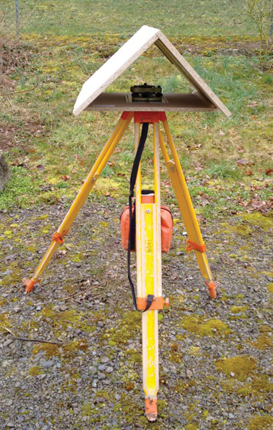
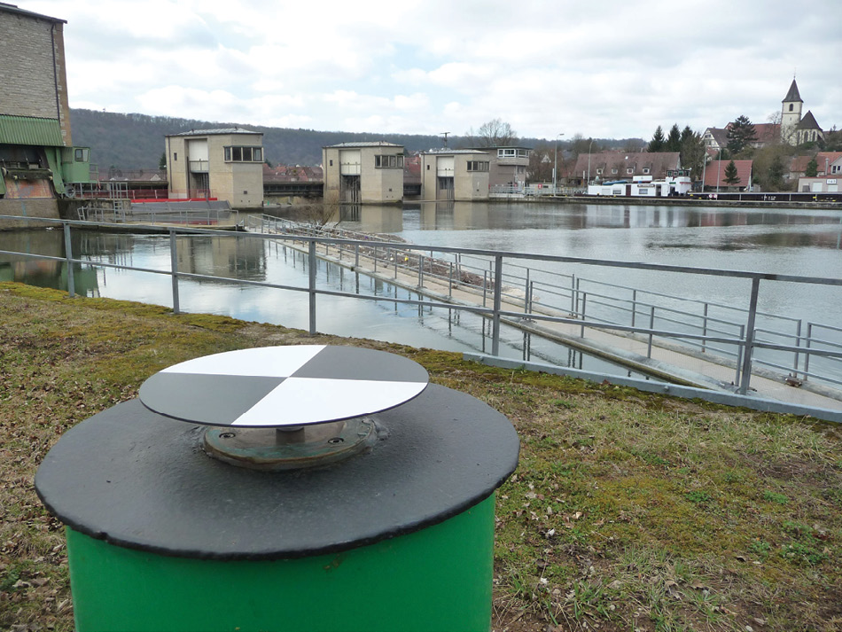 Figure 4: Ship lock and photogrammetric control plane (PCP) on a pillar and lidar control plane (LCP).
At the time of our first flights, no UAV platforms were available that combined a lidar system with a dedicated medium-format photogrammetric mapping camera. Thus, for our earlier experiment in March 2019 we used a RIEGL RiCopter octocopter, which combined a RIEGL VUX-1LR lidar sensor with two oblique-looking Sony Alpha 6000 cameras. In the original concept of the platform, these cameras were intended only to provide RGB color values for the respective lidar points. For such applications, the rather large GSD of 1.5-3 cm at a flying height of 50 m above ground and the rather low radiometric quality of the cameras are sufficient. However, this limits the accuracy of the AAT, which is an integral part of the desired hybrid georeferencing approach.
Triggered by the advantages of joint data collection, commercial platforms are now becoming available, which provide both a lidar system and a medium-format photogrammetric camera. One example is the UAV platform of the company Skyability, which integrates the photogrammetric Phase One iXM-RS150F camera with a RIEGL VUX-1UAV laser scanner and a precise Applanix AP 20 GNSS/IMU unit. This system was used for our flight campaign in March 2021.
As shown in Figure 3, our test flights comprised 52 longitudinal (i.e. north-south) strips, together with six diagonal strips to cover the steep wooded slope in the south-eastern corner of the area. The extra flight lines with diagonal X-shaped trajectories were captured for further stabilization of lidar data processing. With a flying speed of 4 m/s, a nominal flying altitude of 53 m above ground level, a strip width of 20 m, a pulse repetition rate of 550 kHz, a scan line rate of 80 Hz, and a scanner field-of-view (FoV) of 70°, the resulting mean laser pulse density is 300-400 points/m² per strip and about 1300 points/m² for the entire flight block due to the nominal side overlap of 50% as well as the diagonal strips. The laser footprint diameter on the ground is less than 3 cm; the ranging accuracy, as reported in the data sheet of the sensor, is 10 mm.
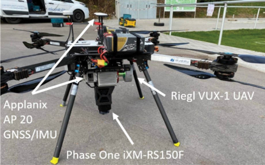
Figure 5: UAV platform with RIEGL VUX-1 UAV scanner, Applanix AP 20 GNSS/IMU unit and Phase One iXM-RS150F camera.
Georeferencing of lidar and image data
During acquisition of lidar data, the measurements of the inertial navigation system and the laser scanner are time-stamped. In post-processing, the IMU and GNSS measurements are combined, using a Kalman filter, into a trajectory, which provides the position and attitude of the platform over time. The polar elements, i.e. ranges and angles, are determined for each laser shot during data acquisition. Based on the trajectory, the scanner’s mounting calibration and the polar measurements of the laser scanner, we calculate the 3D coordinates of each detected laser echo by direct georeferencing. Any error in the estimated trajectory, the mounting calibration, i.e. the position and orientation offset between the estimated trajectory and the scanner’s own coordinate system, or the scanner’s measurements will cause an offset between point clouds of different flight strips in overlapping areas. Respective discrepancies are detected within standard quality control procedures. If the deviations exceed acceptable limits, a typical lidar workflow also includes a strip adjustment to minimize the offsets between the strips. We apply the method presented by Glira et al. (2016), as implemented in the software system OPALS. Within a sophisticated calibration procedure, the six parameters of the mounting calibration (lever arm and boresight misalignment), a global datum shift, as well as trajectory corrections are estimated to minimize the discrepancies defined as point-to-plane distances within the overlap area of pairs of flight strips. To support absolute orientation, the LCPs are additionally considered within this step. Two different solutions for the trajectory correction by the lidar strip adjustment are feasible: (i) the bias correction model considers a constant offset (Δx, Δy, Δz, Δroll, Δpitch, Δyaw) applied to the original trajectory solution of each individual strip; or (ii) a spline model can additionally model time-dependent corrections for each of these six parameters by cubic spline curves. This adds much more flexibility to further minimize the discrepancies between overlapping strips. However, the inherent disadvantage of overfitting by splines can potentially produce block deformations like bending.
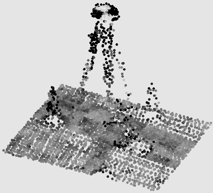
Figure 6: Lidar point cloud at a PCP.
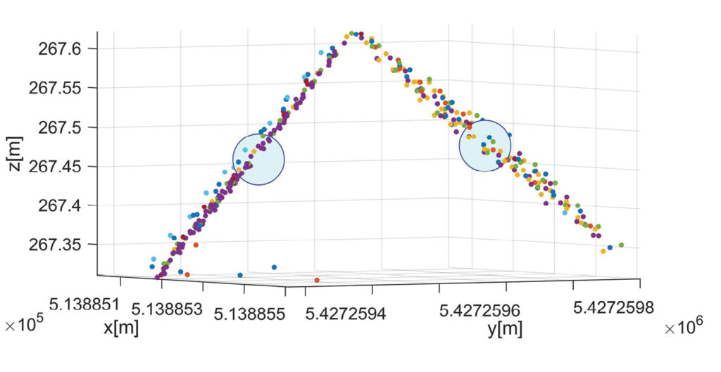
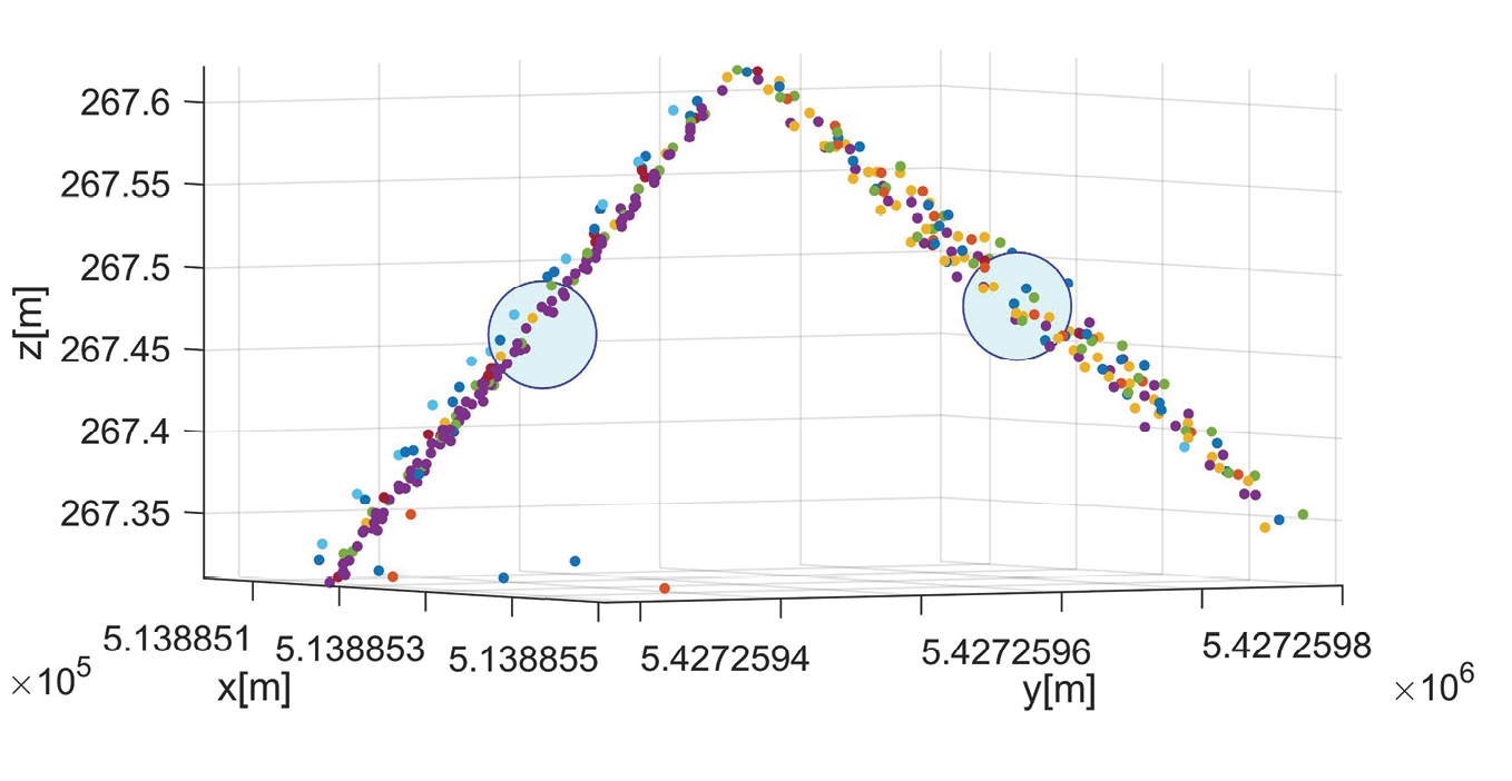
Figure 6 depicts a point cloud at a checkerboard target of a photogrammetric control plane (PCP). Since these signals are oriented horizontally, they only provide point-to-plane differences in the vertical direction. For this reason, they are used only as check points for the vertical component during our investigations on lidar georeferencing. In contrast, the two segments of the lidar control plane (LCP) are inclined by 45°. Hence, the respective point-to-plane differences have both vertical and horizontal components. During georeferencing of the lidar block, the LCPs can be used as both control and check points. Figure 7 shows the lidar point cloud in the vicinity of two LCPs. The respective reference point is depicted in green; the color of the lidar cloud is defined by the respective lidar strip. Each plane of the LCP features an area of 0.32 m2, which results in about 350 lidar points to compute the best fitting plane estimated from the neighboring points of the lidar strips. In this example, the visual interpretation already shows a good fit between points of different lidar strips. Obviously, the deviation to the point of reference is of the same order as the precision of the lidar range measurements, which is given as 5 mm for the VUX-1 UAV system used. For our flight campaign in March 2021, the standard deviation of the residual deviations for the bias solution was 0.92 cm at the PCPs used as check point information. This corresponds very well to the standard deviation of 0.95 cm for the flight campaign in March 2019.

Figure 7: Lidar point cloud for two different LCPs. The center of gravity from the signal is indicated by a blue circle. Lidar point clouds are colored according to the corresponding lidar strip.
 Hybrid georeferencing by joint orientation of lidar and aerial images
The hybrid georeferencing of lidar and aerial images is an extension of the traditional lidar strip adjustment with additional observations from the AAT of image blocks (Glira et al., 2019). Usually, this bundle block adjustment estimates the respective camera parameters from corresponding pixel coordinates of overlapping images, while the object coordinates of these tie points are a by-product. Within the hybrid orientation approach, tie points’ object coordinates from the AAT are re-used to establish correspondences between the lidar and the image block, while the resulting discrepancies are minimized within a global adjustment procedure. In this respect, hybrid orientation adds additional observations and thus constraints to lidar strip adjustments. During hybrid adjustment, both laser scanner and camera can be fully re-calibrated by estimating their interior calibration and mounting parameters (lever arm, boresight angles). Furthermore, systematic measurement errors of the flight trajectory can be corrected individually for each flight strip, by either a constant bias for position and orientation parameters or a spline model for time-dependent corrections. Thus, integrating tie point observations from bundle block adjustment significantly stabilizes the trajectory correction.
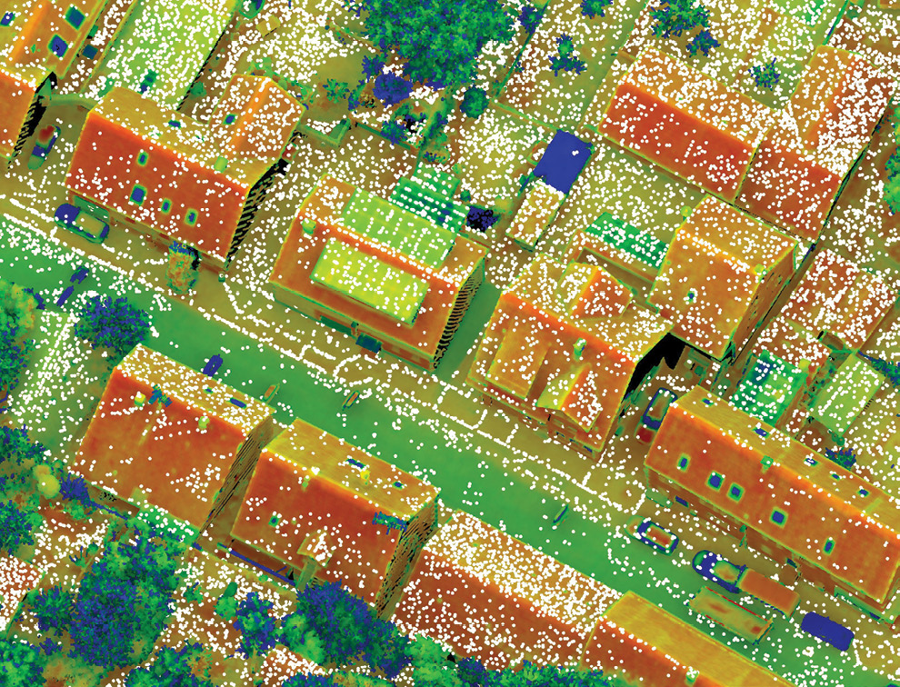
Figure 8: Lidar points coloured by reflectance and photogrammetric tie points (white) for the March 2019 epoch (bottom) and the March 2021 epoch (top).
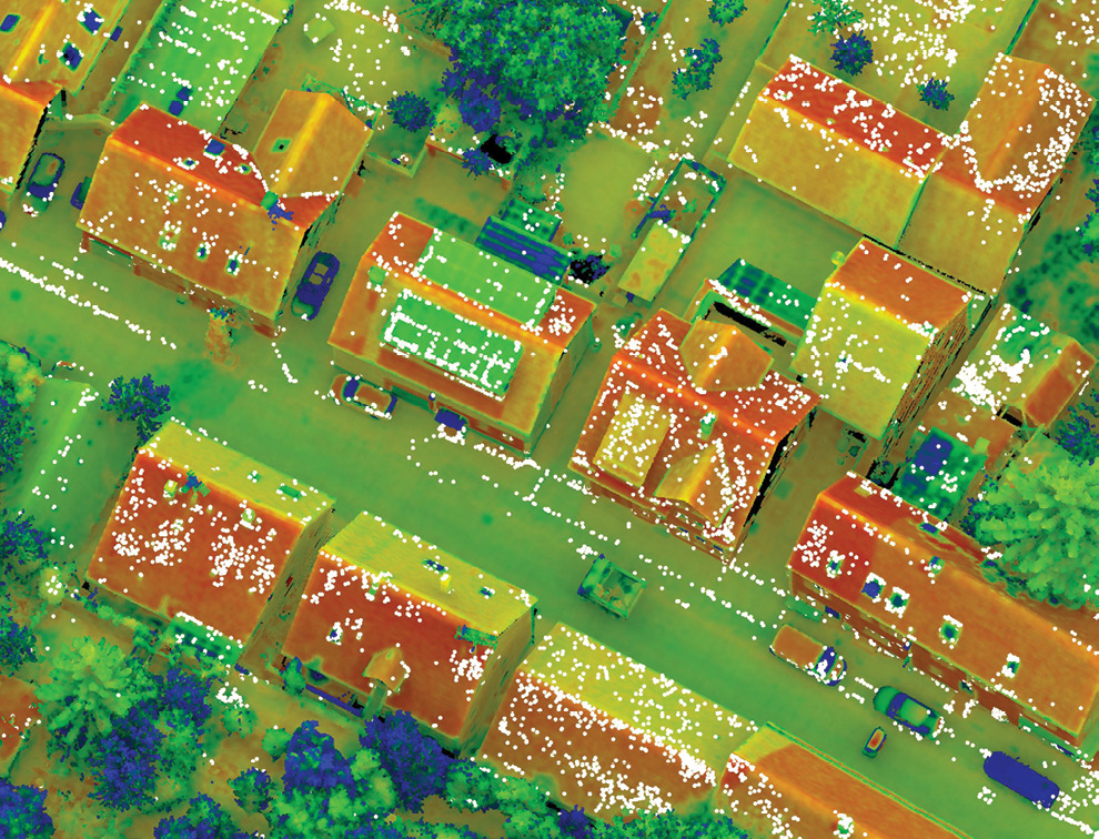
Figure 8 gives an example for the photogrammetric tie points in white and the corresponding lidar points, coloured by reflectance. As discussed by Glira et al. (2019), problems in providing correspondences between points from image matching and lidar can occur from their different properties. To guarantee a suitable accuracy we used only tie points observed in at least three images with a maximum reprojection error of three pixels. In general, tie point accuracy is defined by the respective bundle block adjustment, which is influenced by the geometry of the image block and the image quality. This is the reason why fewer points are available for the campaign in March 2019 compared to the campaign in March 2021, shown on the left and right of Figure 8, respectively. In March 2019 only the rather low-quality Sony Alpha 6000 camera was available, while in 2021 image collection was performed by the medium-format Phase One camera.
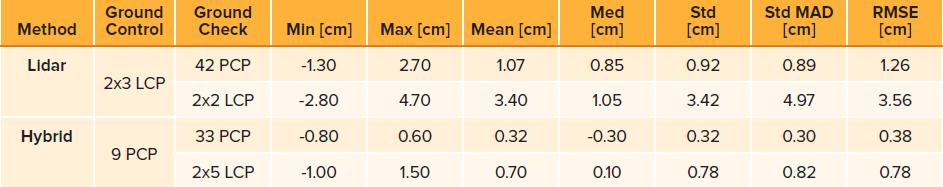
Table 1: Error measures for the flight March 2019 with Sony Alpha camera integrated to the lidar system.
Bundle block adjustment of the Sony Alpha images resulted in differences at independent check points between 5.2 cm (maximum) and 1.2 cm (minimum), with a mean RMSE of 2.5 cm, which was within the range of the GSD of 1.5-3 cm of the captured oblique images. However, the integration of information from that image block into hybrid adjustment resulted in a considerable improvement of the georeferencing results, which is shown in Table 1. While the upper part provides accuracy measures for the lidar-only processing, the lower part gives the respective accuracies for hybrid adjustment. The respective accuracy values were computed from point-to-plane differences between georeferenced lidar point cloud and signalized targets, i.e., the PCPs and the LCPs. Since each LCP consists of two planes, i.e. provides two point-to-plane measures, the five LCPs used as check points during hybrid georeferencing provide 2×5 LCP measurements in Table 1. With respective differences Δ we compute the mean of absolute difference, the standard deviation, the robust standard deviation, i.e. the Median Absolute and the root mean square error. As is visible, accuracy values of hybrid adjustment could be improved by a factor of three compared to lidar strip adjustment.
Despite these promising results based on the Sony Alpha imagery, their validity is limited by the relatively small number of signalized points used as check point information. For hybrid georeferencing 33 horizontally oriented PCPs were available to check for vertical accuracies of the georeferenced point cloud, whereas vertical and horizontal differences, as provided by the LCPs, were limited to five signals. In combination with the availability of an improved camera system, this was our motivation for the additional test flight in March 2021.
Example images of a PCP and LCP as captured by the Phase One iXM-RS150 camera during our flight campaign in March 2021 are given in Figure 9. The 50 mm optics and the selected flying height above ground of 53 m result in a GSD of around 4 mm.

Figure 9: Examples cropped from a Phase One image with PCP and LCP.
Figure 10 shows the distribution of check and control points in the extended test area as well as the color-coded differences between the georeferenced lidar point cloud and the signalized targets. Table 2 summarizes the respective accuracy measures at the photogrammetric targets (PCPs) and lidar targets (LCP). Profile points signalized on the streets provided additional differences in vertical direction as height check points (HCPs). The upper part of Table 2 gives the results for the standard lidar-only processing, whereas the lower part summarizes the results for hybrid georeferencing. For hybrid georeferencing, the RMS error is 5.8 mm for the vertical component at the PCPs and 6.9 mm for the inclined LCPs. As for the precision, the more robust values are 3.0 mm for the vertical component and 2.2 mm for the inclined surfaces. These results confirm and improve our earlier results presented in Table 1. Obviously, the use of a medium-format photogrammetric camera increases the accuracy of hybrid georeferencing. For the March 2019 flight, we evaluated 4550 images at a GSD of 2.3 cm and lidar points at a density of 989 pts/m2 measured with a lidar range accuracy of 15 mm during hybrid georeferencing. The corresponding numbers for the March 2021 flight are 3754 images at a GSD of 5 mm with lidar density of 1368 pts/m2 measured with 10 mm range accuracy. In principle, the increased image resolution for the March 2021 flight should improve the accuracy of hybrid georeferencing even more compared to the March 2019 result. Compared to that flight, we increased the number of signalized check points to improve the overall coverage of our test site. During the evaluation of the 2021 flight, we noticed some larger deviations at those additional points signalized on tripods. However, we kept them in our overall accuracy considerations, despite the fact that this could result in too pessimistic numbers.
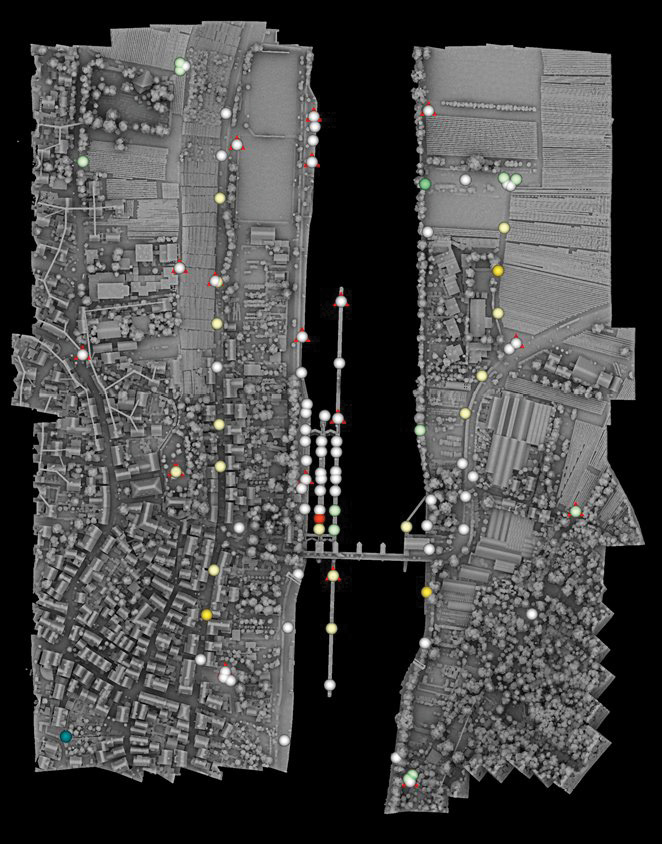
Figure 10: Colour coded differences between georeferenced lidar point cloud and signalized targets for the flight March 2021. Checkerboards used as GCPs are marked by red triangles.
In this context, it should be noted that the coordinate accuracy of the signalized points is already of the order of the accuracy of our hybrid georeferencing. These coordinates are provided from terrestrial measurement, i.e. static GNSS or tacheometry for the horizontal and levelling for the vertical component. Thus, hybrid georeferencing provides lidar point clouds from UAV platforms at accuracies which so far were only available from terrestrial measurement.
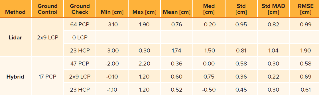
Table 2: Error measures for the flight March 2021 with Phase One camera integrated to the lidar system.
Deformation monitoring based on different epochs
The ship lock and the surrounding area of Hessigheim which has been covered by our test flights is subject to potential subsidence, caused by the geological structure underground (Kauther and Schulze, 2015). The temporal behavior and magnitude of this deformation process are determined by the responsible authority twice a year. This classical monitoring application is based on large-scale tacheometric and high-precision leveling measurements. By these means, significant deformations of the order of about 10 mm/year were identified at several locations in the past. Although these pointwise terrestrial measurement techniques proved to be highly accurate and reliable, the data collection often causes great effort and financial burden. In particular, the necessity of large-scale monitoring of the area surrounding the ship lock represents one of the key cost factors in this context. Besides economic issues, a pointwise monitoring strategy always carries the risk that small-scale deformations are not captured by the network of monitoring points. To come up with an alternative to such a pointwise monitoring strategy, the German Federal Institute of Hydrology (Bundesanstalt für Gewässerkunde, BfG) as the responsible authority funded our research on area-covering UAV-based data collection.
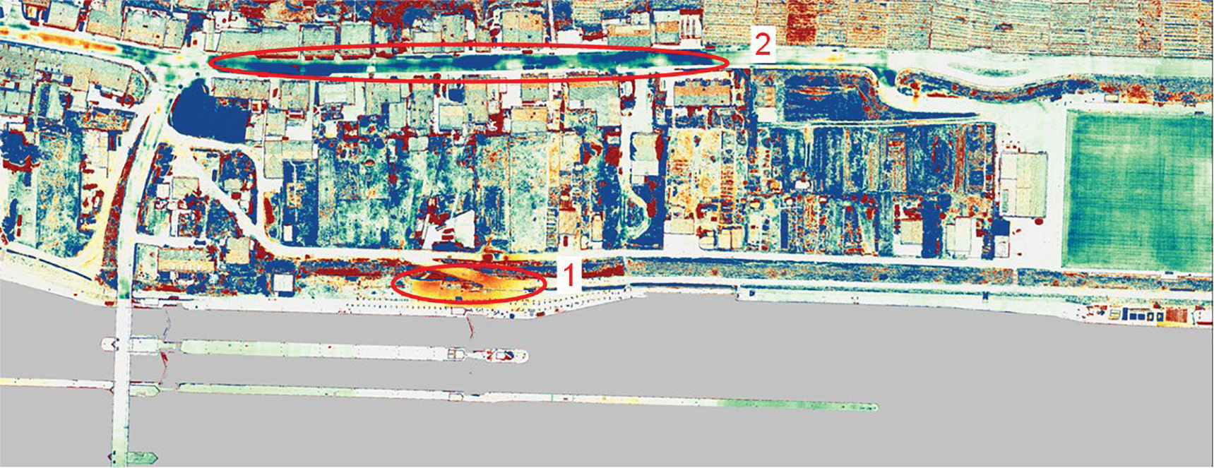
Figure 11: Computed differences of lidar point clouds between epoch March 2021 and epoch March 2019. Marked areas at elevation changes due to subsidence (1) and road surface construction (2).
Figure 11 depicts the computed differences between the point clouds from the measurement campaign in March 2021 and epoch March 2019. The marked area (1) in the immediate vicinity of the ship lock shows differences due to geological subsidence. These could be verified based on prior knowledge of the deformation processes, taken from the terrestrial in-situ measurements. The detected elevation changes at area (2) are due to construction and maintenance work of the road surfaces in the village of Hessigheim. These were performed in summer 2020, i.e. between our measured epochs. One main advantage of airborne lidar is its capability for vegetation penetration, i.e. through trees. However, measurements in low vegetation such as grass result in a mixed signal, i.e. are influenced by the current grass height. Obviously, this is the reason for the elevation differences at vegetated areas visible in Figure 11. In contrast to stable street areas, slight elevation differences are also visible at building roofs. These differences at the inclined roof areas result from remaining georeferencing errors for the horizontal coordinates of the respective 3D point cloud. We assume that these errors mainly occur at the measurement campaign in March 2019, when the accuracy of hybrid georeferencing was limited by the comparably low quality of the Sony Alpha images.
Nevertheless, our results demonstrate the potential of UAV-based data collection to monitor the occurring displacement rates of 6-10 mm/year by applying a suitable sensor setup and hybrid georeferencing. Smaller deformations in the range of only 1 to 2 mm, however, are still beyond detectability. Since such height changes can already be of particular interest, UAV-based monitoring will be integrated with classical and well-established geodetic surveys in future projects. These will apply annual flight missions to detect deformations over larger areas, followed by a more targeted initiation of expensive terrestrial in-situ measurements.
Conclusion
Our investigations on hybrid georeferencing of images and lidar clearly demonstrate the potential of UAV-based data collection to provide dense 3D point clouds at sub-centimeter accuracy. Compared to lidar-only processing, hybrid georeferencing improved the vertical accuracy (RMS) from 9.9 mm to 5.9 mm for our March 2021 flight and from 1.26 cm to 3.8 mm for the March 2019 flight. This enables applications like deformation monitoring, which up to now were feasible only with terrestrial geodetic engineering techniques. In principle, separate platforms can be applied to collect lidar and image data in order to simplify data collection by small and lightweight UAV systems. However, our investigations proved the advantage of joint data collection from a single platform, which constrains the georeferencing process to a joint trajectory for both sensors. Furthermore, contemporaneous data collection simplifies the required matching between lidar measures and tie points from AAT as the most important prerequisite for hybrid georeferencing. Since hybrid adjustment jointly aligns the lidar and image block, ground control can be limited to standard photogrammetric signals, while dedicated lidar control planes are no longer required. This is considered as another main advantage of the hybrid adjustment, as time-consuming terrestrial measurements can be reduced. These benefits were already demonstrated by our first investigations, which applied relatively simple Sony Alpha cameras viewing obliquely. However, the full potential of hybrid georeferencing could be proved using high-quality nadir images as captured by a photogrammetric Phase One camera. Our configuration captured imagery at a GSD of approximately 4 mm, which resulted in lidar georeferencing accuracies of 5.9 mm RMS by hybrid georeferencing.
In addition to high geometric accuracy of the respective point clouds, hybrid adjustment also provides precise co-registration of image and lidar data. This is for example required if MVS is supported by additional lidar measures to enhance the 3D reconstruction process. Such photogrammetric software systems typically generate 3D meshes as an alternative representation to unordered set of 3D points. These meshes are graphs consisting of vertices, edges, and faces that provide explicit adjacency information. The main differences between meshes and point clouds are the availability of high-resolution textures and the reduced number of entities, which is for example beneficial for visualization. Furthermore, 3D meshes are very suitable to integrate information from both lidar and imagery, which is an important advantage both for geometric and semantic information extraction. As an example, semantic segmentation considerably benefits if both lidar echo characteristics and high-resolution imagery are available during feature extraction. This was our motivation to provide the 3D point clouds and meshes as captured during our project in Hessigheim for a benchmark on semantic segmentation (Kölle et. al., 2021). This benchmark includes our multi-temporal lidar point cloud and 3D mesh data sets which have been labelled into 11 classes in order to allow interested researchers to test their own methods and algorithms on semantic segmentation for geospatial applications. From our point of view, such applications will considerably increase the demand for joint collection of airborne lidar and imagery and thus the need for hybrid georeferencing as an important processing step.
Acknowledgement
Considerable parts of the research presented in this paper were funded within a project granted by the German Federal Institute of Hydrology (BfG) in Koblenz.
Bibliography
Glira, P., Pfeifer, N. and Mandlburger, G., 2016. Rigorous strip adjustment of UAV-based la-serscanning data including time dependent correction of trajectory errors, Photogrammetric Engineering & Remote Sensing, 82(12): 945–954.
Glira, P., Pfeifer, N., and Mandlburger, G., 2019. Hybrid orientation of airborne lidar point clouds and aerial images, ISPRS Ann. Photogramm. Remote Sens. Spatial Inf. Sci., IV-2/W5, URL: https://doi.org/10.5194/isprs-annals-IV-2-W5-567-2019.
Haala, N., Kölle, M., Cramer, M., Laupheimer, D. and Zimmermann, F., 2022. Hybrid georeferencing of images and lidar data for UAV-based point cloud collection at millimetre accuracy, ISPRS Open Journal of Photogrammetry and Remote Sensing, Volume 4, April 2022, Article 100014, ISSN 2667-3932, https://doi.org/10.1016/j.ophoto.2022.100014.
Kauther, R., and Schulze, R., 2015. Detection of subsidence affecting civil engineering structures by using satellite InSAR, Proceedings of the Ninth Symposium on Field Measurements in Geomechanics, Australian Centre for Geomechanics, pp. 207-218.
Kölle, M., Laupheimer, D., Schmohl, S., Haala, N., Rottensteiner, F., Wegner, J.D and Ledoux, H., 2021. The Hessigheim 3D (H3D) benchmark on semantic segmentation of high-resolution 3d point clouds and textured meshes from UAV lidar and multi-view-stereo, ISPRS Open Journal of Photogrammetry and Remote Sensing, Volume 1, October 2021, Article 100001, ISSN 2667-3932, https://doi.org/10.1016/j.ophoto.2021.100001.
 Norbert Haala is Professor at the Institute for Photogrammmetry, University of Stuttgart (ifp), where he is responsible for research and teaching in photogrammetric computer vision and image processing. Currently he chairs the ISPRS working group on Point Cloud Generation and Processing and is chairman of EuroSDR Commission 2 on Modelling, Integration and Processing.
 Michael Kölle holds a MSc in geodesy and geoinformatics from the University of Stuttgart. As a member of the geoinformatics group at ifp, he is currently working on his PhD. His main research interests focus on combining paid crowdsourcing and machine-learning techniques such as Active Learning for generating high-quality training data, especially in the context of 3D point clouds.
 Michael Cramer is a senior lecturer at ifp. He has many years of experience in the field of sensor georeferencing and photogrammetric sensors. In addition he serves as secretary of the German Society of Photogrammetry, Remote Sensing and Geoinformation (DGPF).