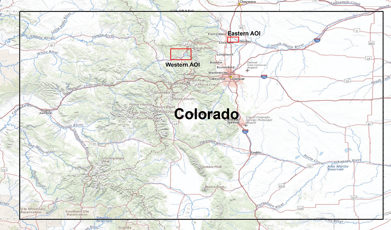
Figure 1: Location of AOIs.
The 3D Elevation Program (3DEP) is a partnership program with many state, local, and Federal partners, managed by the U.S. Geological Survey (USGS) to respond to growing needs for high-quality topographic data and for a wide range of other three-dimensional (3D) representations of the natural and constructed features in the U.S. 3DEP informs critical decisions that are made across the nation every day that depend on elevation data, ranging from immediate safety of life, property, and environment to long-term planning for infrastructure projects. Our goal is to complete acquisition of nationwide lidar (IfSAR in Alaska) by 2023 to provide the first-ever national baseline of consistent high-resolution elevation data – both bare earth and 3D point clouds – collected in a timeframe of less than a decade. The first full year of 3DEP production began in 2016 and by the writing of this article almost 78% of the nation has elevation data available or in progress that meets 3DEP specifications for high accuracy and resolution. 3DEP must also continue to look forward to the challenges of completing nationwide coverage and meeting growing needs for higher quality data, repeat coverage, and new products and services.
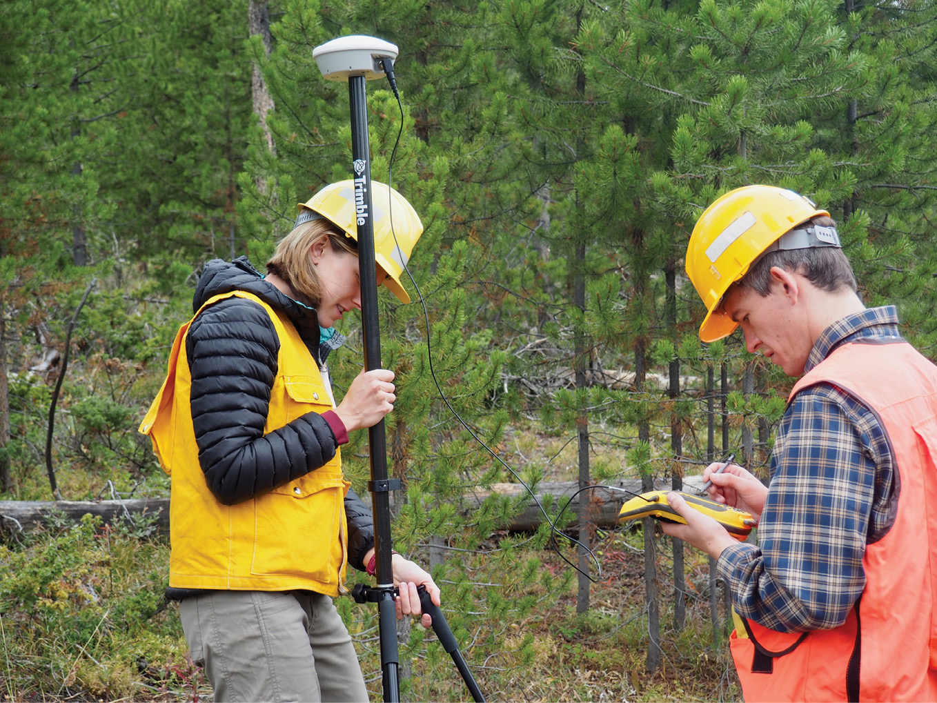
Figure 2: USFS researchers collecting field data. Credit: Gabe Bellante
The National Agriculture Imagery Program (NAIP) acquires aerial imagery during the agricultural growing seasons in the continental US. A primary goal of NAIP is to make digital orthophotography available to governmental agencies and the public within a year of acquisition. NAIP is administered by the Farm Service Agency (FSA) of the U.S. Department of Agriculture (USDA) through the Aerial Photography Field Office (FSA-APFO) in Salt Lake City, Utah. This “leaf-on” imagery serves as a base layer for GIS programs in FSA’s County Service Centers and is used to maintain the Common Land Unit (CLU) boundaries.
These two Federal programs, with their distinct needs and goals, have been discussing how to align data acquisitions for potential cost savings. Both NAIP and 3DEP members had been contacted about the potential of a new sensor, the Leica CountryMapper from Leica Geosystems, part of Hexagon1, to collect imagery and lidar simultaneously for both NAIP and 3DEP. The Leica CountryMapper sensor is currently in development and its specifications are not yet publicly available; but it has been claimed to have the potential to collect data that satisfies both 3DEP and NAIP requirements in a single collection. The Leica CountryMapper is a hybrid sensor that collects imagery and lidar data simultaneously, based on the lidar system from the Leica TerrainMapper and the camera system from the Leica ADS100. This pilot project was designed to help 3DEP determine if this sensor has the potential to meet current and future 3DEP topographic lidar collection requirements, ideally at the same altitudes and leaf-on times that NAIP is flown. The field surveys were performed to evaluate the 3D absolute and relative accuracy of the airborne Leica CountryMapper lidar and to determine if the data met 3DEP specifications.
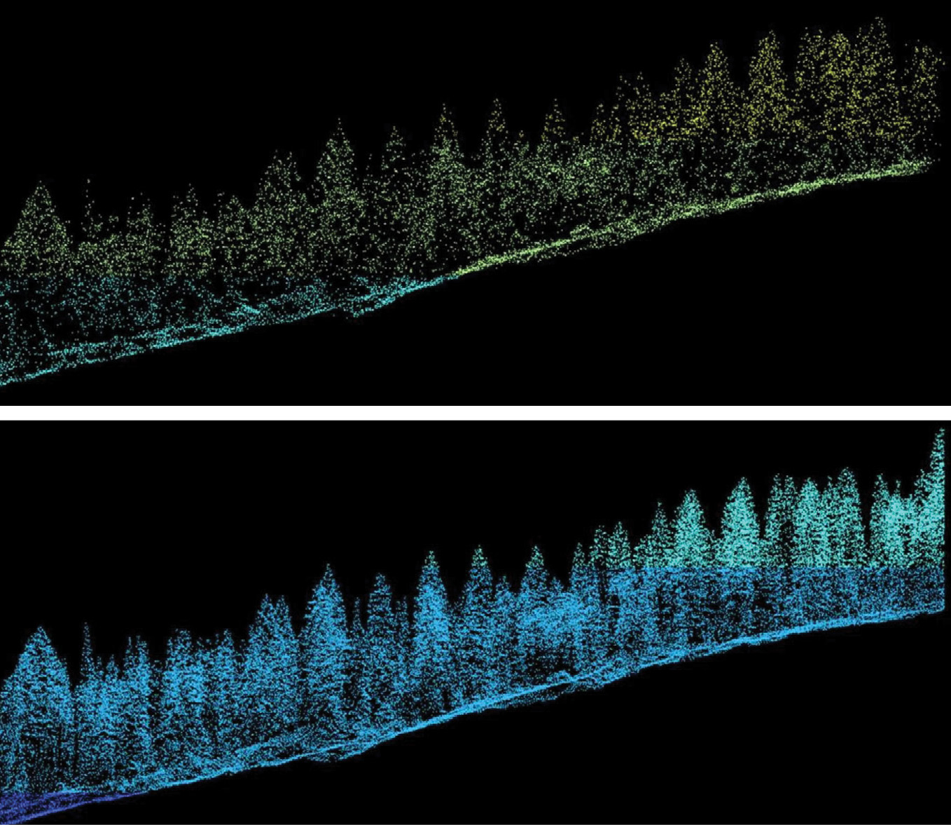
Figure 3: A profile comparison of the 2010 Grand County lidar data (top) and the 2019 Leica CountryMapper data (bottom).
To test the claims that a sensor could meet both NAIP and 3DEP requirements simultaneously, a multiagency group consisting of USGS, FSA, the USDA Natural Resource Conservation Service (NRCS), Bureau of Land Management (BLM), National Park Service (NPS) and U.S. Forest Service (USFS) began working together to analyze a single collection for the various needs. NAIP was confident about the sensor’s ability to meet its imagery needs, so the focus of this study was on the quality and characteristics of the resultant lidar.
The airborne data acquisition for this pilot project was funded by the NRCS National Geospatial Center of Excellence (NGCE) as an add-on to the NAIP acquisition, working with FSA-APFO, now part of the Farm Production and Conservation (FPAC) office. These USDA agencies collaborated to plan and execute the pilot project. Early on, USDA reached out to USGS, USFS, BLM, NPS, and other Federal 3DEP partners to guide and support the project with technical expertise and field work. The latter is a crucial component of the pilot project, enabling the comparison of ground observations with measurements from the remotely sensed imagery and lidar.
This paper discusses the various methods different agencies used to evaluate the same dataset and presents some results. It is our hope that in the future a multiagency evaluation approach to test multiple needs from a single dataset will become more commonplace.
See PDF for more graphics.
Site selection
Two pilot areas of interest (AOIs) were selected to be flown in north-central Colorado over two different physical settings in order to evaluate the system’s performance (Figure 1). The western AOI included land managed by BLM, NPS and USFS. The forested land in the western AOI primarily consists of a mixture of lodgepole pine, quaking aspen, Engelmann spruce and subalpine fir. The mountain pine beetle had a devastating impact on the forest, killing many of the lodgepole pines and leaving many of them standing dead or downed. The eastern AOI included agricultural and urban areas.
Hexagon acquired data for this project, operating at an altitude of 3.6 km, a speed of 180 knots, a pulse repetition frequency of 750 KHz and a scan rate of 112 Hz, giving an imagery product of 20 cm ground sample distance and a pulse density of 2.9 points per square meter (ppsm). Its elliptical scan pattern allowed for the separation of the point cloud into forward and backward scanned groups, which enabled intraswath difference analysis.
USFS analyses
The objectives of USFS for analyzing data from the sensor included: 1) evaluate the quality of the lidar data to see if it meets Lidar Base Specification Quality Level 2 (QL2) density specifications (2 ppsm); 2) assess the quality of standard forestry derivatives, such as canopy height and cover rasters; and 3) collect field data and test the efficacy of using these data for forest inventory modeling.
USFS analyzed the Leica CountryMapper data for the western AOI alongside lidar that was previously collected in 2010 in Grand County, Colorado. It derived canopy height (1-meter) and cover (10-meter) rasters from both datasets using USFS FUSION software (version 3.80), then compared the quality of the outputs and interpreted the changes that occurred between 2010 and 2019. Three USFS researchers spent four days collecting 28 forest inventory plots. Field measurements included plot center locations at sub-meter accuracy and individual tree measurements including tree species, diameter, live/dead status, and tree height samples (Figure 2). USFS used these field data in combination with the lidar data to create linear regression models for a total of nine forest inventory metrics (Mitchell et al., 2015; Tenneson et al., 2018).
Based on analysis by USFS, the density and vertical distribution of the 2019 Leica CountryMapper point-cloud data appeared to be an improvement over the 2010 Grand County data. Figure 3 shows a side profile view of a mixed conifer forest, illustrating the higher point density of the Leica CountryMapper data, which results in a better representation of individual trees and understory vegetation.
To evaluate the pulse density of the Leica CountryMapper data, USFS produced first-return rasters at two different scales: cell sizes of 1 m and 10 m. For both approaches, the Leica CountryMapper data met or exceeded 2 ppsm, with 99.5% of cells at the 10-m scale and 97.7% at the 1-m scale meeting that threshold. We found that the average first-return pulse density was approximately 5.36 ppsm.
In addition to evaluating point-cloud density, USFS assessed the quality of canopy height and cover rasters derived from the Leica CountryMapper data. These datasets are commonly used in USFS to inform applications such as tree-stand delineation, habitat mapping, and canopy gap analyses. The 2019 Leica CountryMapper canopy height raster, shown on the right-hand side of Figure 4, represents the above ground height of all objects in the study area and captures the detail of individual tree crowns. In Figure 4, the 2010 and 2019 rasters look very different because of the extensive lodgepole pine mortality throughout the study area. The upper right portions of the images in Figure 4 are mainly lodgepole pine, and their narrow crowns in the 2019 image are characteristic of the mountain pine beetle damage in this area. The trees that have largely remained the same are aspen: they are tall, with relatively large crowns, and can be seen throughout the middle and upper left of both images. In this area, the Leica CountryMapper data appears to represent high-quality canopy height information, as individual crowns are distinguishable and many small-diameter tree crowns are captured in the raster.
Figure 5 juxtaposes the 2010 and 2019 canopy height raster data in a dense aspen stand. In both years, individual aspen crowns are hard to distinguish because the trees have similar heights and the canopies are very tightly knit. The 2019 raster has more gaps within the aspen canopy, which could represent natural gaps during the growing season, or gaps because the data were collected around the time that leaves start falling from aspen stands at this elevation (~9160 feet). The dieback of lodgepole pines, located on the right side of the figure for both years, is also evident in the canopy height data.
Figures 6 and 7 show a zoomed-in view of the 2010 and 2019 canopy cover rasters. Based on a qualitative assessment, the canopy cover values are reasonable, capturing both densely and sparsely forested areas well. Moreover, there are no obvious, widespread acquisition artifacts in the 2019 raster. Such artifacts are related to the variable point density from different flight and scan lines rather than real patterns on the landscape and would appear as parallel lines in the data. These artifacts are relatively common in acquisitions not collected with the flight line overlap specifications that are ideal for forestry derivatives.
Figure 8 shows the differenced canopy cover raster that was created by subtracting the 2010 from the 2019 canopy cover raster. The positive values in red represent areas where the 2019 canopy cover percent was higher than 2010. Conversely, the negative values in green represent areas where 2010 canopy cover percent was higher than 2019. The red pixels are largely associated with areas of forest growth where the trees were below 2 m in height in 2010. The distinct patches of green are primarily associated with lodgepole mortality: the trees in those patches appear dead in the 2010 imagery, and many of them had fallen or been cut down by 2019.
The final component of the USFS analysis was linear regression modeling of forest inventory metrics, including basal area and board foot volume, two metrics that are not directly measurable from a lidar point cloud. USFS produced a total of nine forest inventory rasters for the entire western AOI, most of which had statistically significant R2 values greater than 0.60 (see Table 1). Figure 9 shows results for the merchantable cubic foot volume and basal area models, which were modeled with R2 values of 0.82 and 0.71 respectively. Despite the limited number of plots collected and a non-rigorous sample design for the field plot placement, the results of the USFS analysis were very promising. The forest inventory models largely had high R2 values and a qualitative comparison of the modeled data with NAIP showed good correspondence in relative values of the modeled data with the differences in forest density apparent in the NAIP imagery.
Overall, USFS determined that the data exceeded QL2 density specifications at both the 100-m² and 1-m² scales. Nearly 98% of pixels in the 1-m² pulse density assessment met the 2-ppsm threshold, indicating a consistency in pulse density across the study area. The lidar-derived canopy height and cover rasters are suitable for a wide range of forestry applications. The canopy cover values aligned well with 2019 NAIP, and the data showed no prominent acquisition artifacts, which appear as stripes in rasters and are relatively common in acquisitions without 100% flightline overlap. Similarly, the canopy height data appear to be high quality, although the level of detail in individual crowns, particularly in densely forested areas, could be improved. Crown dimensions in some of the dense aspen stands appeared lacking, but this may be due to the tightly knit canopies and similar heights of those stands.
While the number and locations of sample plots were not ideal, the forest inventory modeling results from this project demonstrate the efficacy of using the Leica CountryMapper data to model forest inventory parameters that are not directly measurable from the point cloud. Even with the limited number of plots collected and the less than ideal plot placement, models performed relatively well. Basal area and quadratic mean diameter models, metrics commonly used by foresters and timber crews throughout the USFS to describe forest stocks, performed well, with R² values of 0.71 and 0.70 respectively. The biomass (R²=٠.٣٤) and board foot volume (R²=٠.٥٤) metrics performed poorly, however, which may be due to a few factors, including the high levels of mortality in the study area, the accuracy of allometric equations for the study area, and the limited number of plots.
USGS analyses
Field data were collected by USGS in two different field campaigns. The first took place in the western AOI, near Granby, Colorado, on 8–11 September 2019. The second occurred in the eastern AOI, east of Fort Collins, Colorado, on 18–20 November 2019.
The western AOI included six field sites. Four were on land managed by BLM, where BLM had established seven field plots (Figure 10). One site was on land managed by USFS and one was at Windy Gap Wildlife Viewing Area. The eastern AOI included four field sites. The first consisted of two houses in the southeastern portion of Fort Collins, Colorado. The remaining sites were Chimney Park, Windsor Main Park, and Eastman Park, all within Windsor, Colorado.
USGS collected GNSS data using a Trimble R8 Model 2 base station with a TDL-450H external data radio, in combination with a Trimble R8 Model 2 rover and a Trimble R8 Model 3 rover. The Trimble GNSS equipment has a horizontal accuracy of ±1 cm plus 1 part per million (ppm) root mean square (RMS) 2 cm and a vertical accuracy of ±2 cm plus 1 ppm RMS 3 cm.
USGS also used an Optech ILRIS 3D laser scanner equipped with a pan/tilt base to conduct the terrestrial laser scans. The Optech ILRIS 3D has a raw range accuracy of 7 mm at 100 m and a raw positional accuracy of 8 mm at 100 m. It has a 40o x 40o field of view and scans at the near-infrared wavelength of 1535 nm. Using the pan/tilt base allows the scanner to capture up to 10 FOV scan sections, covering 360o horizontally with 2o of horizontal overlap on each end of a scan section. USGS also collected UAS data for analyses, but for the purpose of this article results are not included. All survey data were published, including the UAS data, and can be found at https://doi.org/10.5066/P9CPDWUU (Irwin et al., 2020).
To investigate the quality of the data, USGS assessed absolute accuracy compared to survey ground data as well as absolute and relative accuracy tests using a new method that involves intraswath and interswath comparisons (Kim et al., 2020). Assessing absolute vertical accuracy is a practical choice, because assessing horizontal accuracy is difficult with point cloud data. Checkpoints were surveyed in clear, open areas (which typically produce only single lidar returns) for non-vegetated vertical accuracy (NVA) assessment. Checkpoints for vegetated vertical accuracy (VVA) assessment were surveyed in vegetated areas, which typically produce multiple returns. Both the Root Mean Square Error RMSEZ and 95th percentile methodologies for NVA and VVA respectively are currently widely accepted in standard practice and have been proven to work well for typical elevation datasets derived from current technologies. Checkpoint survey areas were homogeneous and in areas of gentle slope (<10°).
Intraswath and interswath analyses are another category of accuracy analysis. Intraswath analysis utilizes point cloud data from a single swath. For instance, smooth surface precision measures the consistency of the elevation along a smooth planar object from a single swath, because surface precision is determined mainly by the laser ranging uncertainty and scanner stability. When two lidar swaths overlap and lidar point cloud features extracted from planar features of one swath are compared to the other, it is a relative interswath difference, and the RMS difference can be determined. Interswath overlap consistency reveals the fundamental quality of the lidar point cloud because it establishes the quality and accuracy limits of all downstream data and products. Boresighting or other calibration errors result in substantial interswath differences. USGS used a point cloud-based interswath difference method using geometric features (such as three-plane objects described below) in the overlapping area from two swaths to do the comparisons.
By finding planar surfaces (such as building roofs) with enough sampled points, we can generate a virtual plane through these points. A three-plane geometrical feature creates a unique intersection point at the top. An intersection point determined from a high-accuracy reference dataset over the same features (e.g. TLS) can be used to evaluate the accuracy of an airborne lidar point cloud, such as the Leica CountryMapper data. An intersection point can be computed for planes in both the airborne data and the reference data (Figure 11). The difference between two intersection points represents the error between the two lidar point clouds in three dimensions. We call this the “generic three-plane” method. We tested this methodology comparing TLS data to the Leica CountryMapper data on the eastern AOI over several houses (Figure 12).
We found multifaceted roof objects, then calculated conjugate intersection points from the reference TLS data and from the airborne data. The differences gave error vectors (Dx, Dy, Dz) that were compiled into a table detailed by Kim et al. (2020), documenting the mean shift and RMSE for each axis. The mean shift along the X-axis is substantially large (~20 cm) when compared to the shifts along the Y-axis (7–8 cm) and the Z-axis (3–6 cm).
To evaluate intraswath smooth surface precision, USGS used a park office building in Eastman Park, Windsor, Colorado, as shown in Figure 13. The example point cloud from the roof plane marked by the yellow cross was sampled. The histogram of the normal distance to the plane is shown, with a RMSE of 2.2 cm. Of the 60 plane features extracted in the 3D absolute accuracy study, each yielded a smooth surface precision value, and the average was 2.5 cm.
The 2.2 cm RMSE intraswath smooth surface precision value (Figure 13) is excellent based on the USGS QL2 requirement (<6 cm). Very small intraswath differences between opposite scan directions were observed. Again, compared to USGS QL2 requirements (<6 cm), these results indicate there was minimal systematic error and the quality of the Leica CountryMapper boresighting was high. The differences between two intersection points in the interswath analysis (all 2 cm or less) were also very small, considering the USGS QL2 requirement (<8 cm).
USGS also performed NVA analysis of Leica CountryMapper lidar point clouds on three sites in the eastern AOI. The NVA mean was approximately 2 cm and the RMSE was less than 3 cm, which is also very low compared to the USGS QL2 requirement (<10 cm). Since the mean value (~2 cm) is computed by subtracting the lidar point elevations from the ground truth point elevations, it means that the airborne lidar data are approximately 2 cm lower than the GNSS-measured “true” elevation.
The VVA analysis of the UAS lidar data showed a reasonable mean shift and RMSEZ. The negative VVA mean values are understandable because the lidar return from the low vegetation is a little bit above the ground surface where the survey pole would rest. The VVA mean values from airborne lidar ranged from -3 cm to -8 cm, depending on the BLM sites. The RMSEZ values were 3–5 cm, which is well within the USGS QL2 requirement (<10 cm).
Conclusion
Both USFS and USGS analyses of the Leica CountryMapper data show promising results. All the results appeared to satisfy the USGS QL2 requirements, although some of the point cloud vector-based methods presented here are new and are different from the raster-based methods suggested in the Lidar Base Specification. USGS used a novel 3D absolute accuracy assessment method, based on geometric features, as a potential future standard accuracy assessment practice. Despite some limitations, USGS demonstrated that the practice of assessing the 3D absolute accuracy of lidar point clouds was a viable option during the NAIP/3DEP campaign and will continue to work on improving ground-survey protocols. USFS found the Leica CountryMapper data to be suitable for producing a wide range of high-quality forestry rasters, including canopy height, canopy cover and more complex forest inventory models.
Remember that this pilot project was flown at altitudes to support 20-cm NAIP imagery collection, so no conclusions can be made about the claims of meeting 3DEP requirements from altitudes needed to collect 1-meter imagery for entire states. Also, while this pilot project did pass the test of collecting data leaf-on, these areas in Northern Colorado are sparse in terms of vegetation cover. We hope to attempt another pilot project in the future at higher altitudes over much denser vegetation.
By the time this article is published, many of the specifications of the sensor on which these analyses were based may be obsolete as sensor improvements are continuously being made. The methodology and division of labor to ensure that multiple Federal teams can investigate various requirements from a single dataset, however, provided a very useful exercise. In addition to ensuring that 3DEP technical requirements are met, substantial planning and coordination between agencies is still needed to determine if the technology can be made operational for 3DEP.
References
Irwin, J.R., A. Sampath, M. Kim, M.A. Bauer, M.A. Burgess, S. Park and J.J. Danielson, 2020, CountryMapper Sensor Validation Survey Data: U.S. Geological Survey data release, https://doi.org/10.5066/P9CPDWUU.
Kim, M., S. Park, J. Irwin, C. McCormick, J. Danielson, G. Stensaas, A. Sampath, M. Bauer and M. Burgess, 2020. Positional accuracy assessment of lidar point cloud from NAIP/3DEP pilot project, Remote Sensing, 12(12): 1974, 20 pp.
Mitchell, B., M. Beaty, R. Reynolds, T. Mellin, A.T. Hudak, A. Schaaf and H. Fisk, 2015. Creating LiDAR canopy structure layers and inventory models for evaluating northern goshawk habitat quality, Report number: RSAC-10070-RPT1, Salt Lake City, Utah: United Stated Department of Agriculture, Forest Service, Remote Sensing Applications Center, 21 pp.
Tenneson, K., M.S. Patterson, T. Mellin, M. Nigrelli, P. Joria and B. Mitchell, 2018. Development of a regional lidar-derived above-ground biomass model with Bayesian model averaging for use in ponderosa pine and mixed conifer forests in Arizona and New Mexico, USA, Remote Sensing, 10(3): 442, 28 pp.
Jason Stoker, Elevation Science and Application Lead, U.S. Geological Survey (USGS), National Geospatial Program, Reston, Virginia.
Aparajithan Sampath, contractor to U.S. Geological Survey (USGS) Earth Resources Observation and Science (EROS) Center, Sioux Falls, South Dakota.
Minsu Kim, contractor to U.S. Geological Survey (USGS) Earth Resources Observation and Science (EROS) Center, Sioux Falls, South Dakota.
Jeff Irwin, Geographer, U.S. Geological Survey (USGS) Earth Resources Observation and Science (EROS) Center, Sioux Falls, South Dakota.
Eric Rounds , Remote Sensing Project Manager, RedCastle Resources; on-site contractor at USDA Forest Service, Geospatial Technology and Applications Center, Salt Lake City, Utah.
Joshua Heyer PhD, Geospatial Specialist, RedCastle Resources; on-site contractor to the USDA Forest Service, Geospatial Technology and Applications Center, Salt Lake City, Utah.
Julie Davenport, Lidar and Photogrammetry Specialist, U.S. Forest Service, Geospatial Technology and Applications Center, Salt Lake City, Utah.
Gabe Bellante, U.S. Forest Service, Geospatial Technology and Applications Center, Salt Lake City, Utah.
Tony Kimmet, National Imagery Leader, U.S. Department of Agriculture-Farm Production and Conservation-Business Center – Geospatial Enterprise Operation, Fort Worth, Texas.
Collin McCormick, Section Chief, U.S. Department of Agriculture-Farm Production and Conservation-Business Center – Geospatial Enterprise Operation, Fort Worth, Texas.
John Mootz, Former Imagery Program Manager, U.S. Department of Agriculture-Farm Production and Conservation-Business Center – Geospatial Enterprise Operation, Salt Lake City, Utah.
1 Any use of trade, firm, or product names is for descriptive purposes only and does not imply endorsement by the U.S. Government.