Seagrass’s role in Florida
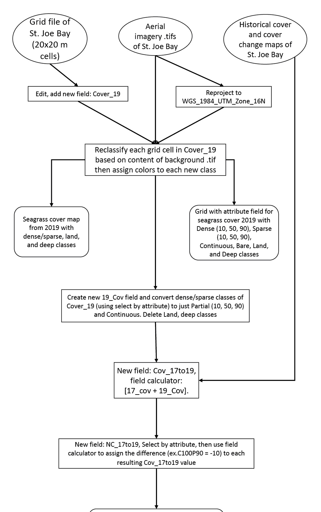
Figure 1: Flowchart of GIS procedure used for mapping and data collection. Circles represent input data layers, rectangles represent processing, while rounded rectangles represent produced map layers.
Contrary to their common name, seagrasses are technically marine monocotyledons, which means that they are a flowering plant that moved into the water around 70-100 million years ago. Despite their low species diversity and distinct physiological characteristics, seagrasses have successfully colonized every ocean, save for the poles (Orth et al., 2006).
Their importance is derived from the priceless natural services that these plants provide for the anthropocentric world as well as entire ecosystems. As a result, these grasses are worth over $19,000 per hectare, making them the third most valuable ecosystem in the world. Indeed, they are intrinsically priceless, as they promote and directly support much of the biodiversity that is characteristic of coastal and marine ecosystems. They are “ecosystem engineers” due to their strength and “coastal canaries” due to their vulnerability.
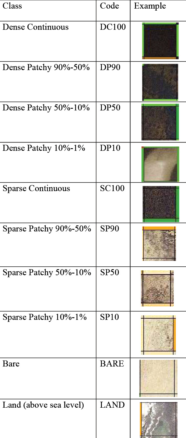
Figure 2: Photointerpretation key with examples from imagery
Seagrasses are representatives of the health and status of both their own and surrounding ecosystems, including human environments and economies. Seagrasses also support marine life by acting directly as a food source, or as a nursery and habitat for a diverse array of species. Commercial as well as recreational inshore fishing in Florida relies on many of these same species, such as tarpon, snapper, and grouper (Matz, 2015). Tourism centered around species which are considered megafaunas, such as manatees and sea turtles, is equally important to the economy of Florida (FWC, undated).
Since seagrasses are so important, they also experience a wide array of stressors and disturbances. These include but are not limited to herbivores, competing producers, tides, air exposure, hurricanes, storm surges, water quality, and turbidity (ibid.). Perhaps the greatest global threat to seagrasses is humans and their various exploits. The world’s population has historically resided, developed, and polluted near the coast, including bays and estuaries—the areas where seagrasses are most abundant and biogeographically important to the environment (Griffiths et al., 2020).
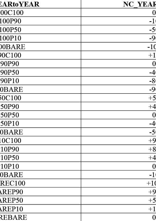
Figure 3: Conversion key for all possible combinations of percentage cover change with corresponding percent change value.
St. Joseph Bay “is dominated by large monospecific stands of Thalassia testudinum interspersed with smaller patches of Halodule wrightii, unvegetated sand flats, and small amounts of Syringodium filiforme” (Heck and Valentine, 1991, 217). The variegated sea urchin, “L. variegatus, previously observed defoliating large expanses of seagrass in the northern Gulf of Mexico, is commonly found within vegetated areas of St. Joseph Bay with population densities as high as 140 individuals/m2” (ibid., 216). These events are classified as overgrazing when urchin populations overwhelm and impair ecosystem services. The causes include eutrophication due to runoff from various point and non-point sources, overfishing of the sea urchin’s natural predators, and rising water temperatures. A 2019 study of sea urchin populations in St. Joseph Bay after Hurricane Michael suggests that vegetated areas averaged about 13-14 individuals/m2 (Challener et al., 2019). The same study noted that sea urchins here are “remarkably” resistant even to intense storms. They also noted that smaller individuals were likely swept away by the strong wave action during the hurricane and left the larger individuals behind to repopulate.
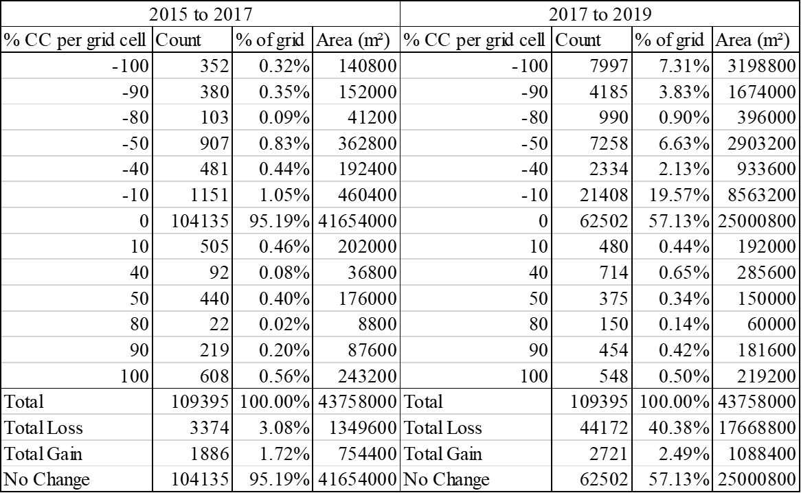
Figure 4: Results of cover change analysis for the two most recent studies, displaying the frequency, percent of grid, and area of seagrass that experienced varying degrees of gain or loss.
While all these factors influence the status, health, and productivity of seagrass meadows, this study focuses on quantifying seagrass loss after Hurricane Michael as well as potentially related sea urchin grazing. Hurricane Michael in October 2018 is ranked as the third most intense of all recorded hurricanes to have struck the continental United States up to that point. It traveled north up the Gulf of Mexico and hit the Big Bend region of Florida’s panhandle, including St. Joseph Bay, causing 30 billion dollars in catastrophic damage to multiple coastal towns. While property and infrastructure losses have been calculated, the effect of this storm on the environment and its natural ecosystem services has yet to be fully assessed. To quantify and analyze the seagrass loss caused by these processes, seagrass meadows in the waters of St. Joseph Bay were mapped using aerial imagery taken in March 2019.
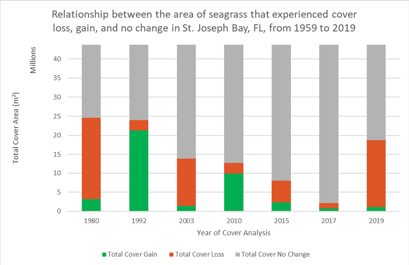
Figure 5: Percent of seagrass that experienced cumulative cover gain, loss, and no change 1959-2019
Three main layer groups were manipulated within Esri ArcMap 10.3.1 for this analysis. Kucera International provided over 40 aerial imagery tiles, taken with a multispectral sensor at high resolution (10215 x 10215 pixels) with 8-bits-per-band depth. These were added to the working ArcMap document, one layer per .tif file. The tiles do not overlap each other and cover the full extent of the bay, so they function as the first layer group that is manipulated in this study. The second layer group consists of six different 20 x 20 m grid shapefiles with both cover and cover change attributes for each cover study completed by the Fish and Wildlife Research Institute (FWRI). These will be merged later with the Cover19 grid (the numerals refer to 2019, the date of the data). The third, topmost layer is a 20 x 20 m grid shapefile with an empty Cover19 field. The properties of this grid are changed so there is no color fill to the cells, and the aerial imagery can be clearly seen beneath. This layer is to be edited the most and will contain the completed cover change analysis maps. The first and third layers remain active during data collection while the second and third layers remain active during data processing and analysis. All layer groups were projected to the geographic coordinate system WGS 1984 UTM Zone 16N. The workflow, process, and methods for this analysis are depicted in Figure 1.
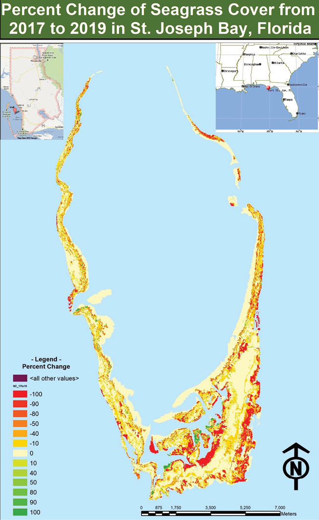
Figure 6: Map of percent cover change per grid cell 2017-2019.
Currently there is not an accurate automated method to detect the presence of seagrass and then classify it as such—only manual photointerpretation and supervised, semi-automated methods. Lidar and remote sensing abilities are limited due to the functioning of light underwater with suspended particles, turbidity, and swaying motion of seagrass that is dictated by underwater currents. This study area includes a very complex water column, since it is located in the salty Gulf of Mexico, so for these reasons aerial photography was utilized in this study and not lidar. As topobathymetric lidar capabilities increase and intertwine with neural networks and deep learning, it is highly likely that the current method will be accurately replicated without a user-intensive process and instead utilize multiple sensors, models and algorithms at once to automate the process.
For this study, I hand digitized all of St. Joseph Bay’s seagrass meadows in the aforementioned empty 20 x 20 m grid shapefile’s Cover19 attribute field. The grid consists of approximately 109,395 cells, each with an area of 400 m2, and follows the interior perimeter of St. Joseph Bay, including the littoral zone where seagrass meadows are located and distributed. Each cell was objectively assigned one classification label using the classification table in Figure 2.
Techniques to achieve this quickly and efficiently are made possible by ArcMap, as it is much too time-consuming and therefore inefficient to classify one cell at a time. These tools include highlighting, de-selecting highlighting, and the field/classification calculator within the attribute table.
After the preliminary manual classification was completed, an additional field was added to the grid’s table. The purpose of this is to re-classify the ‘Cover19’ field, so it has the same classifications as the historical seagrass cover maps in St. Joseph Bay and can then be compared. The real difference is that the reclassification takes away the subclasses of dense versus sparse for eight classes in total. The second layer group contained the historical cover shapefiles from FWRI and was spatially joined with the newly filled and converted shapefile so that the cover data from the years 1959, 1980, 1992, 2003, 2010, 2015, 2017, and now 2019 exist all in the same shapefile under the same data point classification key. From there, the calculations of cover change were made within the attribute table for this map document on ArcMap by combining two years of cover data at a time (example: 17_Cover and 19_Cover).
There are 25 resulting classifications or values of this calculation, which correspond to the 25 possible combinations of cover change codes that represent the approximate total cover lost or gained within every grid cell in the shapefile for two consecutive cover studies. These 25 possible combinations are then treated like subtractive equations, with 25 differences and numerical values to represent the difference in the percent cover change between studies. Figure 3 depicts this relationship. These values are then added to the attribute table of the grid so they can be displayed to map the change between two studies. The field calculator was used to fill each attribute with the numerical value, as it had been used to populate the preliminary 2019 cover data.
Finally, the frequency, area of cover, and subsequent percent of total cover for each of the 25 class/value combinations of cover change can be calculated for any study year. The frequency of grid cells that experienced any percent of cover change was determined using the ‘Select by Attribute’ feature for each numerical value of percent change. Then each frequency was multiplied by the area of one grid cell (400 m²) to calculate the total area of seagrass that experienced any of the possible percent changes per grid cell. These calculations were then divided by the total area of the grid that contained bare sand or seagrass (109,395 grid cells = 43,758,000 m² or 43.758 km2), which excludes classifications of land, deep water, and missing imagery, to find the percent of the total study area that experienced each possible percent change. Figure 4 compares the percent cover categories of the 2017-2019 results with that of 2015-2017.
By using an interpretation-based mapping and calculation process, this study found that, between 2017 and 2019, approximately 17.6688 km² of seagrass cover experienced a decline while only 1.0884 km² experienced cover gain. This recorded cover loss is greater than that of previous cover studies except for that between 1959 and 1980. As displayed in Figures 5 and 6, this study found that 40.38% of all seagrass meadows in St. Joseph Bay experienced decline from 2017-2019, 2.49% experienced cover gain and 57.13% did not experience cover change. 7.31% of all seagrass meadows experienced a total loss in 2017-2019.
Thus seagrass in St. Joseph Bay experienced a significant decline between 2017 and 2019, likely caused by a combination of multiple stressors present in the area, including but not limited to Hurricane Michael, recreational boat propeller scarring, sea urchin grazing, nutrient runoff, water clarity, and phytoplankton. Earlier FWRI seagrass mapping efforts determined that all but one of these stressors are either episodic or increasing, with propeller scarring determined to be extensive (Yarbro and Carlson, 2016). The maps created from this study, using imagery from 2019, indicate continued evidence and extent of thinning.
Future work
This study is subject to human error during manual classification and photointerpretation, related to the limitation of the grid’s resolution. Each grid cell or pixel is 20 x 20 m, so all calculations are approximations. Without historical data before 1959-1980, it is impossible to determine longer-term trends. There remains a need for restoration and/or conservation, since seagrass beds are so valuable ecologically and economically on both global and local scales. Using the data, statistics and maps, areas of highest concern and vulnerability can be identified as part of the third Seagrass Integrated Mapping and Monitoring Program Mapping and Monitoring Report produced by FWRI. Seagrass mapping and monitoring is crucial for the effective ecosystem management of St. Joseph Bay.
Allison Senne is an undergraduate at University of South Florida St. Petersburg, majoring in environmental science and policy. She has a minor in geospatial sciences and is completing the honors designation in the Judy Genshaft Honors College at USF. She will graduate in May 2021. She works part-time at the Florida Fish and Wildlife Conservation Commission’s Fish and Wildlife Research Institute in the Seagrass Habitat lab (led by Drs. Laura Yarbro and Paul Carlson) using ArcMap and aerial imagery to map and digitize seagrass meadows in coastal areas of the Florida panhandle.
References
Challener, R., J. B. McClintock, R. Czaja and C. Pomory, 2019. Rapid assessment of post-hurricane Michael impacts on a population of the sea urchin Lytechinus variegatus in seagrass beds of Eagle Harbor, Port Saint Joseph Bay, Florida, Gulf and Caribbean Research, 30(1): SC11-SC16. doi:10.18785/gcr.3001.07.
FWC (Florida Fish and Wildlife Conservation Commission), undated. Seagrass FAQ, https://myfwc.com/research/habitat/seagrasses/information/faq/.
Griffiths, L.L., R.M. Connolly and C.J. Brown, 2020. Critical gaps in seagrass protection reveal the need to address multiple pressures and cumulative impacts, Ocean & Coastal Management, 183, 104946, 1 January 2020. doi:10.1016/j.ocecoaman.2019.104946.
Heck, K.L. and J.F. Valentine, 1991. The role of sea urchin grazing in regulating subtropical seagrass meadows: evidence from field manipulations in the northern Gulf of Mexico, Journal of Experimental Marine Biology and Ecology, 154(2): 215–230. doi:10.1016/0022-0981(91)90165-s.
Matz, H., 2015. Current threats to coastal seagrass ecosystems, Shark Research & Conservation Program, University of Miami, 18 March 2015. https://sharkresearch.rsmas.miami.edu/current-threats-to-coastal-seagrass-ecosystems.
Orth, R.J., T.J.B. Carruthers, W.C. Dennison, C.M. Duarte, J.W. Fourqurean, K.L. Heck, A. Randall Hughes, G.A. Kendrick, W. Judson Kenworthy, S.V. Olyarnik, F.T. Short, M. Waycott, S. L. Williams, 2006. A global crisis for seagrass ecosystems, BioScience, 56(12): 987-996, December 2006. https://doi.org/10.1641/0006-3568(2006)56[987:AGCFSE]2.0.CO;2.
Yarbro, L. A. and P. R. Carlson (eds.), 2016. Seagrass Integrated Mapping and Monitoring Program: Seagrass Integrated Mapping and Monitoring Report No. 2, Fish and Wildlife Research Institute Technical Report TR-17, version 2, 281 pp.