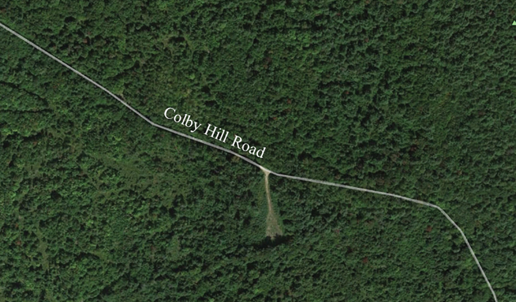
Figure 1: Google Earth image showing the ground in the lidar image (Figure 2) in Henniker, NH to be obscured by the forest canopy. Width of view is 0.67 mile.
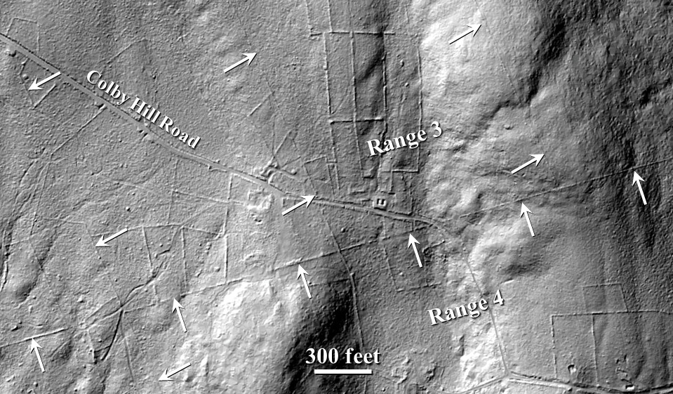
Figure 2: Lidar image from the NH Stone Wall Mapper showing a 0.7-mile segment of the ENE-trending, stone wall-defined boundary between Ranges 3 and 4 in a heavily wooded area (43.1887°N; 71.8789°W) near Colby Hill Road in Henniker, NH. This boundary was laid out by Matthew Patten’s survey team on Thursday, October 5, 1752 using a magnetic compass-bearing of N84°E. The bearing relative to True North is N74.4°E, which yields a magnetic declination of 9.6°W in October 1752. The geomagnetic field model gufm1 also gives a value of 9.6°W for the magnetic declination at this location in late 1752. The NW-trending boundaries for lots # 17 and 18 had a magnetic bearing of N15°W in the original survey. Many other stone walls are also visible in this view, but were not built along the original 1752 boundaries.
My first experience with stone walls was as a young kid (6-10 years old) living in South Deerfield, NH. The family home was the site of an abandoned farmstead consisting of massive stone foundations of quarried granite and stone walls throughout the woods. Decades later while living in a rural setting outside Albany, NY, I renewed my childhood fascination by mapping about 6 miles of stone walls in the nearby woods using a handheld GPS unit. The resulting map showed a complex pattern that made no sense until a 1790 map of property boundaries in the town was located. Upon recognizing the geophysical potential of these stone walls, I mapped 726 miles of stone walls in New Hampshire (312 miles) and New York (414 miles) using old land surveys and lidar images. The results of that work have recently been accepted for publication in the Journal of Geophysical Research: Solid Earth. The title of the article is … Measurements of geomagnetic declination (1685-1910) using land surveys, lidar, and stone walls (scholarsarchive.library.albany.edu/cas_daes_scholar/5).
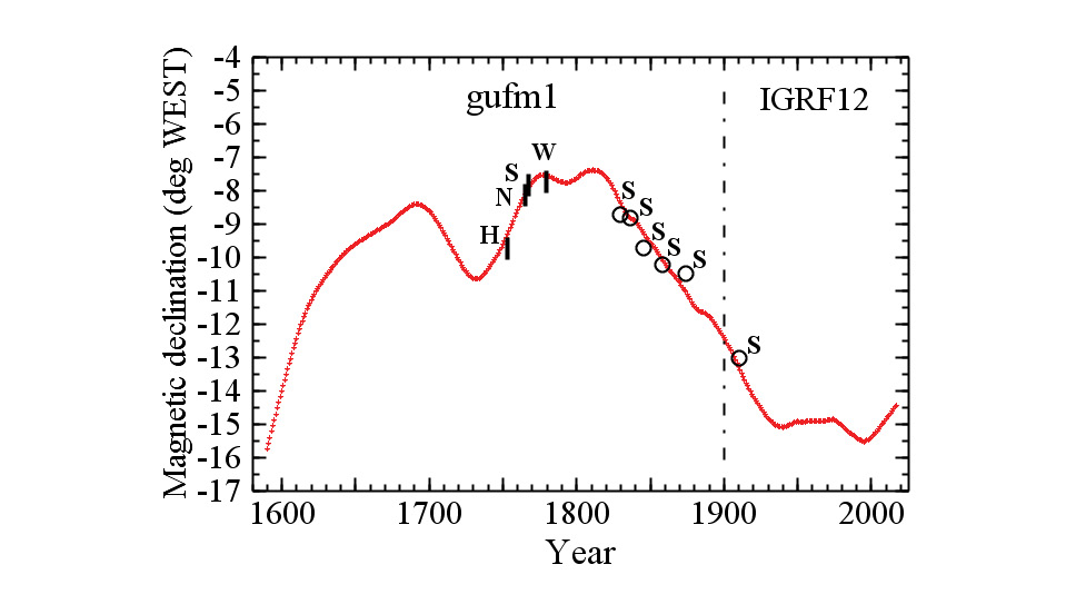
Figure 3: 233 miles of stone wall-defined boundaries in Henniker (H; 41 miles), Nelson (N; 38 miles) Stoddard (S; 141 miles), and Windsor (W; 13 miles) were mapped using lidar images to determine the magnetic declination at those locations based on land surveys conducted in the latter half of the 18th century. Those magnetic declinations are shown plotted against the gufm1 (pre-1900) and IGRF12 (post-1900) geomagnetic models (red curve). With the exception of the time-interval of 1775-1810 for surveys at other localities in New Hampshire and New York that differ from the geomagnetic models by up to 1.5-2.0° eastward, the differences between the declinations inferred from the stonewall-defined boundaries and the geomagnetic models are usually less than 0.5°.
Lidar images with resolutions of about 3 feet are required to locate and map stone walls. The NH Stone Wall Mapper (granit.unh.edu/resourcelibrary/specialtopics/stonewalls/) described by Rick Chormann, State Geologist and Director of the New Hampshire Geological Survey, in the February 2019 issue of the NHLSA Newsletter provides a complete set of processed lidar images for all of New Hampshire. This is a superb resource!
While finding stone walls on lidar images is straightforward, interpreting them is a different matter. Which walls were constructed along property boundaries? When were those property boundaries surveyed? Those two questions consumed most of my effort. Historical literature for each locality (Appendix 1 in JGR article) was needed to ultimately determine the date and magnetic bearings of the original land surveys, especially of townships. New Hampshire has an excellent compilation of that historical information (e.g., volumes by Albert Stillman Batchellor that are available on-line: sos.nh.gov/Papers.aspx). Those searches of the historical literature sometimes led to accounts from 18th century survey teams that had been commissioned to lay out hundreds of ~100-acre lots along range boundaries, many of which are still defined by old stone walls in New Hampshire and New York.
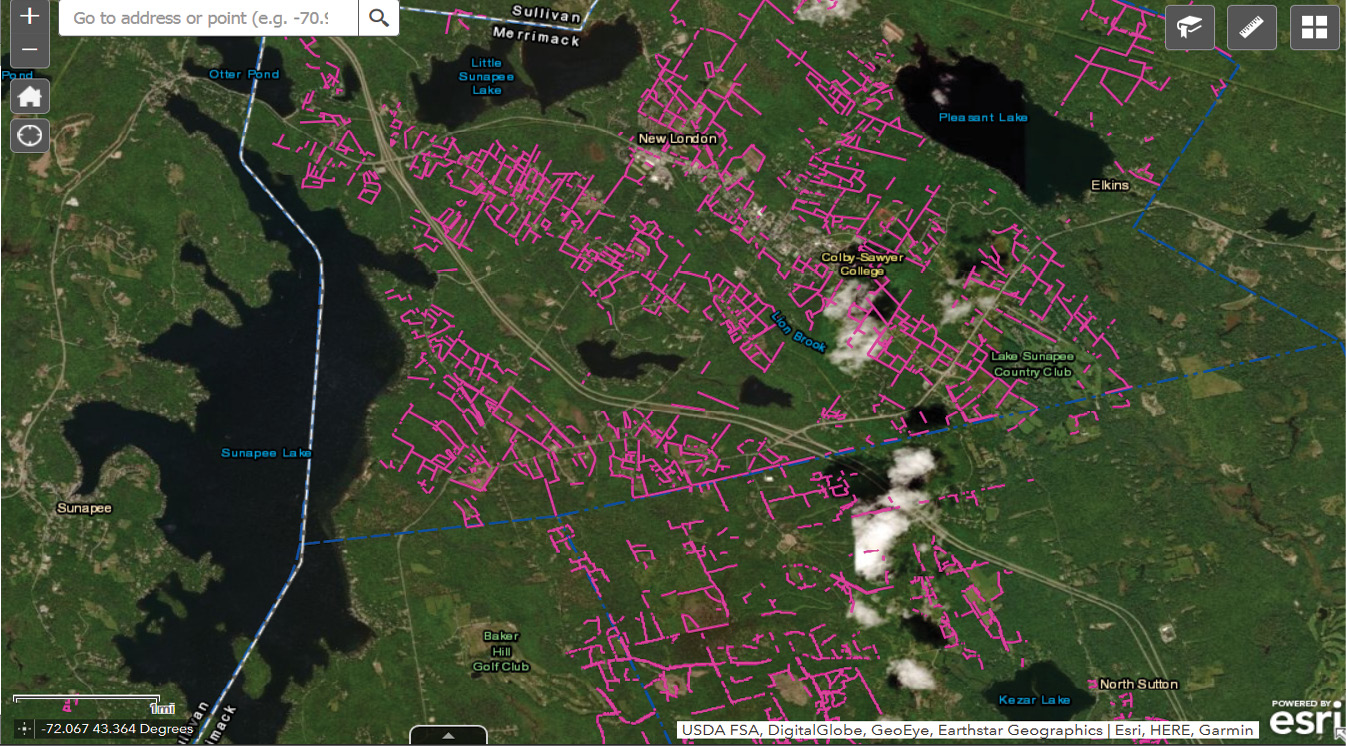
Figure 4: Area in Sullivan and Merrimack counties of New Hampshire with some of the stone walls (pink lines) have been mapped. NH Stone Wall Mapper: granit.unh.edu/resourcelibrary/specialtopics/stonewalls
The diary of Matthew Patten, who was in charge of a metes-and-bounds survey in 1752-1753, described the daily challenges of rough terrain and harsh weather as his team of axmen, chainmen, and surveyors laid out hundreds of lots in 45 miles2 of rugged wilderness in Henniker, NH (L. W. Cogswell, 1880. History of the Town of Henniker, Merrimack County, New Hampshire, from the date of the Canada Grant by the Province of Massachusetts, in 1735, to 1880. Republican Press Association, Concord, NH. 868pp). Using those detailed accounts, it was possible to track the paths of Patten’s survey team along the range boundaries and to identify the team’s location on lidar images during notably difficult times. Such accounts with the lidar images have fascinated public audiences. Figures 1 and 2 shows stone wall-defined boundaries laid out by 1752 surveys in northeastern Henniker.

Figure 5: Lidar image of the same area shown in Figure 3 showing the abundance of stone walls. Most of these stone walls were built by 18th and 19th century farmers, many of whom subsequently left the area. The forests soon reclaimed the fields that had been bordered by stone walls.
Stoddard, NH was fortunate to have a surveyor and dedicated historian, Charles L. Peirce (1874-1963), who generated a detailed map of lots and ranges (stoddardnh.org/about-us/pages/charles-peirce-maps-stoddard) that were laid out in the original survey in 1768-9 and are often defined by stone walls today. Although none of the stone walls are continuous from one side of the town to the other, most can be extrapolated among the current remnants to define a systematic grid. Mapping stone wall-defined boundaries along ranges and lots defined by the original survey in Stoddard, and those in nearby towns, the magnetic declinations at those locations were determined and compared with the current geomagnetic model, gufm1 (ngdc.noaa.gov/geomag-web/#declination). Figure 3 show excellent agreement. However, as documented in the forthcoming JGR paper, a systematic difference of 1.5-2.0° in magnetic declination (i.e., more eastward than gufm1) was found for surveys done in 1775-1810 at other regions of New York and New Hampshire. Local magnetic anomalies in the earth’s crust are not considered the likely cause of the geographic extent, magnitude, and direction of that difference. The gufm1 model apparently needs revision during that time-interval.

Figure 6: Lidar view of area from Figure 4 stone walls (pink lines), eastern portion of Lake Sunapee (left edge) Routes 103A (center), and US Route 89 (upper right corner). Width of view is about 1 mile. NH Stone Wall Mapper: granit.unh.edu/resourcelibrary/specialtopics/stonewalls
In summary, stone walls that were built by the early settlers along boundaries laid out by the original land surveys of New Hampshire townships still exist. With knowledge of the original land surveys and the use of lidar images (NH Stone Wall Mapper), those stone wall-defined boundaries can be distinguished from the myriad of other walls within a township. Although the boundary walls are often intermittent, lidar images allow the original boundaries, where stone walls are absent, to be located between existing stone wall segments by interpolation. Finally, the current geophysical model, gufm1, provides a good description for changes in the magnetic declination since the late 17th century, except for the interval 1775-1810 when the declination was apparently 1.5-2.0° eastward of the gufm1-derived value.
Note: This article appeared in the April issue of the New Hampshire Land Surveyors Association TBM and is reprinted by permission.
John earned a Ph.D. in Geology at Stony Brook University, State University of New York, in 1977. His research was competitively funded by NASA and/or the National Science Foundation (NSF) for nearly 35 years and resulted in 70 professional publications. John served on, and chaired, scientific advisory panels for NASA and NSF, and was the Associate Director of NASA’s Astrobiology Institute, which was multi-institutional research consortium headquartered at Rensselaer Polytechnic Institute. He retired from his academic career at the University at Albany in 2017 at the rank of Distinguished Teaching Professor in the Dept. of Atmospheric and Environmental Sciences and Associate Dean for the College of Arts and Sciences. John and his wife, Susan, are currently residing in Williamsburg, VA.