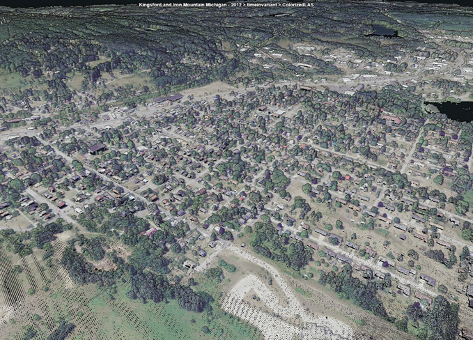
Figure 1: Fused USDA lidar, NAIP imagery
Our company, GeoCue Group, has been doing a lot of work these past two years in the areas of data processing and management running in Amazon Web Services (AWS). There is a game you play with AWS (and other “cloud” vendors) to try to reduce the cost of using the service. It is an interesting fact that cloud architectures represent a compromise between designs optimized for the host architecture/use cases (the science bit) and the goal of minimizing system rental costs (the business bit).
Editor’s note: A PDF of this article as it appeared in the magazine is available HERE.
At any rate, this analysis of our deployments in AWS made me start thinking about the term “data fusion.” We toss this round a lot; in fact, I think one of my previous Random Points random ramblings was on this very subject. Recently, I have come to appreciate a subtle distinction between data fusion and what I will call “analytic fusion”. This distinction matters a lot when you are paying a cost (dollars or time) for moving data.
Traditional data fusion means mixing data from different sources (e.g. sensors) to create a product that is either better than the individual sources alone or is aimed at a special application. The primary goal is to create a new data set that is richer in content than any of the individual source data sets. An example is shown in Figure 1. This is a point cloud from United States Department of Agriculture (USDA) lidar data colorized with image data from the USDA National Agriculture Imagery Program (NAIP). This fused data product was generated in GeoCue’s Earth Sensor Portal, a data management and cataloging system hosted in AWS. This product is creating by populating red-green-blue (and, optionally, near-infrared) data fields in the lidar data (in LAS format) with the interpolated image data from the NAIP. The result is a beautiful, colorized 3D point cloud that is useful in myriad applications. This is the key thought, however when creating a data fusion product, we are not completely sure what will be asked of the result.
Generation of this product requires moving data from the storage location of the NAIP to the storage location of the lidar data. Some NAIP is stored in AWS East Region, whereas most USGS lidar data are stored in AWS West Region. It can cost up to 9 cents per gigabyte to move data between AWS regions, so this is a major consideration when designing a cloud-hosted environment to perform the fusion process.
Analytic fusion, on the other hand, is aimed at using two or more sources of data to answer a specific question. The goal is not to mash the data together to generate a new, richer data set, but rather just to seek solutions to some specific problems that are known a priori. An example might be to use a feature layer containing building footprints and a set of lidar data with classified building points to look for areas of change. Here I am not interested in creating a rich, fused data product but simply an analytic result. To carry out this analysis I might find the centroids of the building footprints as compact X, Y points (I probably do not need the elevations). I could then transport these to the region containing the lidar data. I would then find the difference between the union and intersection of the centroids and the lidar building classes. The result would be a compact set of centroids that represent the change.
The difference between these two processing models can be subtle until you get your cloud services bill! There is an old adage regarding large dataset processing: “move the processor to the data.” This could be quite difficult in complex on-premise physical environments but is generally quite easy in virtualized cloud environments. When playing the game to reduce cost, it can often be useful to extract just the bits you need from each data source and then do the fusion. In the case of colorizing lidar data, we are pretty much stuck. The parts of the data we need to bring together represent the bulk of the size, so just grit your teeth and move the lighter to the heavier (in this example, the image data are “lighter”). Of course, you can play some tricks such as doing any necessary subsampling prior to data transmission. It goes without saying that you always employ a very efficient data compression scheme prior to transmission. And whatever you do, avoid truly bloated data schemas such as KML, XML and GeoJSON when dealing with voluminous data (I guess we have proven that there are, indeed, formats less efficient than ASCII—anyone care to join us in porting Shape to 64 bit?).
As developers, we have always been aware of the cost of processing in terms of storage devices, processing time, user experience and so forth. Actually paying rapidly multiplying pennies for computer and transfer resources brings this to the forefront of design. The bottom line here is that you have a new consideration when designing for metered, virtual environments.