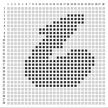
Figure 1: An image of a digit from MNIS
This month I was going to discuss how to fly and process LIDAR data for 27 cents per km2 but Allen (Cheves, the publisher) reminded me that I owe him part 2 of the neural networks discussion. Oh well, must save that processing secret for another time!
Last month I provided a review of the rebirth of the artificial neural network (ANN) as one of the more popular approaches to solving computational problems. In fact, it has become so ubiquitous that off-the-shelf libraries exist, allowing you to quickly roll your own ANN analytic system. Their primary use has been in systems where the problem is classification (dividing things into categories) and the problem space is fuzzy with a lot of training data available. One of the outstanding successes of ANN has been in natural language processing (think Siri, Google, Alexa and so forth).
Of course, our interest is in applying this technology to LIDAR and image processing problems. If you followed part one of this article, you noticed that a bare bones ANN requires an input per pixel. In LIDAR processing, this would be an input per point. Even the little digit recognition problem that I referenced at the end of the article, with its 28 x 28 input images comprising the MNIST data set (see an example digit in Figure 1), requires a whopping 784 input neurons (one per input pixel). This approach will not scale to a real-world LIDAR/image data set.
A critical fact with imagery, LIDAR and other select data types such as speech is they have spatial or temporal coherence. This means that the closer two points are to one another in space or time, the more likely they are to be related to the same feature. Conversely, the further apart, the less likely. This is very easy to visualize in imagery/ LIDAR. If we view, top-down, an image of a rectangular building roof that is 10 m x 20 m in world coordinates, then two pixels more than 22.4 m (the length of the diagonal) apart cannot both be part of the same building roof. We can take advantage of this localization by preprocessing the imagery into blocks. Since, at the end of the day, we are interested in extracting features from the data, we may as well process the data into blocks with enhanced feature primitives (such as edges). The time-tested way to do this is by running filters over the image in an operation called convolution. An example of an edge enhancing filter is shown in Figure 2. If we then subsample these feature blocks (in neural network jargon, this is termed “pooling”) we can reduce the input data size to something more amenable to neural network input.
A block diagram of this series of processing steps is shown in Figure 3. The general flow is to enhance features using various convolution filters into groups of enhance images, subsample these into blocks (“pooling”) and then feed these individual preprocessed pixels (“flattening”) into a conventional artificial neural network. The combined process is termed a Convolutional Neural Network (CNN) even though the preprocessing steps are performed using conventional image processing algorithms. Note that we can actually increase the data size (and usually do) by using not one convolutional filter but a large set that do different things such as “enhance left to right diagonals” “enhance right to left , diagonals” etc. This large collection of , enhanced images is then reduced in the pooling step. This provides a very rich set of distinct features to feed into the conventional ANN.
When processing multispectral imagery, we can use cross channel information in the preprocessing steps (e.g. mix the red and blue channels). When processing LIDAR data, we simply treat the third dimension (e.g. height) as another channel.
The use of CNNs in LIDAR data processing is really in its infancy. We are seeing some prototype applications coming to market but the mainstream use of CNNs in production and analytic processing is still a bit in the future. While CNNs show great promise, they do have some drawbacks. They obviously require tremendous compute resources. This is being addressed by cloud services such as Microsoft Azure and Amazon Web Services who offer ANN engines (such as MXNET) “out-of-the-box.” One current handicap to CNN is the lack of robust training data. Unlike predictive algorithms, a neural network must be fed examples of what it is to detect. If we want to train a CNN to extract buildings, we must have a set of multiple copies of every building we want detected! Over time it is likely that a set of public domain training sets (similar to the idea of MNIST) will become available. This will dramatically accelerate the adoption of useful CNNs for LIDAR processing.
In spite of the drawbacks of CNNs, they show great promise toward solving certain types of recognition problems. Chances are, if you work in LIDAR data from the production or analytic side, a CNN is in your future.